
BIOL-321 · Lesson 5 of 12 · 27 min
Quantitative traits and the response to selection
Many of the traits that matter most in evolution, from body size and flowering time to milk yield and disease risk, vary continuously and are influenced by many genes and by the environment. BIOL-201 introduced heritability and the breeder’s equation, R = h²S, which predicts how much a trait changes in one generation of selection. This lesson builds on that foundation. It looks at how heritability is estimated and what it does and does not mean, how selection on one trait changes others through genetic correlations, what long-term selection experiments reveal and how the polygenic architecture of traits, now visible through genome-wide studies, shapes their evolution.
Partitioning variation
The phenotypic variance of a trait, V_P, can be divided into a genetic part, V_G, and an environmental part, V_E. The genetic part is further split into additive variance, V_A, which comes from the average effects of alleles and makes offspring resemble their parents; dominance variance, V_D, from interactions between alleles at the same locus; and interaction (epistatic) variance, V_I, among loci. Broad-sense heritability is H² = V_G/V_P; narrow-sense heritability, h² = V_A/V_P, is the part that determines the response to selection, because only additive effects are reliably passed from parents to offspring.
| Trait | Typical narrow-sense heritability | Notes |
|---|---|---|
| Human height (European-ancestry samples) | About 0.7–0.8 | High in well-nourished populations |
| Body weight in livestock | About 0.3–0.5 | Breeding targets |
| Milk yield in dairy cattle | About 0.25–0.35 | Large gains from selection since the 1950s |
| Beak depth in Galápagos ground finches | About 0.7–0.8 | Measured by Peter and Rosemary Grant |
| Clutch size in birds | About 0.2–0.4 | Life-history trait |
| Fertility and survival traits | Often below 0.1 | Fitness components tend to have low heritability |
Heritability is often misunderstood. It is a property of a population in a particular environment, not of a trait in general or of an individual. A heritability of 0.8 for height does not mean that 80 per cent of a person’s height is due to genes. It means that, in that population and setting, 80 per cent of the variation among people is due to additive genetic differences. Heritability can change if the environment changes; in a population where some people are malnourished, environmental variance increases and heritability falls. Crucially, high heritability within groups says nothing about the causes of average differences between groups, which may be entirely environmental.
Estimating heritability
The simplest estimate comes from the resemblance of offspring to their parents. If offspring trait values are regressed on the average of their two parents (the midparent), the slope estimates h². Regressing on a single parent gives h²/2. Twin and family studies in humans, animal pedigrees analysed with mixed models (the animal model), and, increasingly, genome data from unrelated individuals all provide estimates.
import numpy as np
rng = np.random.default_rng(321)
# Simulate a trait with additive genetic variance VA = 0.6 and environmental variance VE = 0.4
n = 3000; VA, VE = 0.6, 0.4
a_mother = rng.normal(0, np.sqrt(VA), n); a_father = rng.normal(0, np.sqrt(VA), n)
z_mother = a_mother + rng.normal(0, np.sqrt(VE), n); z_father = a_father + rng.normal(0, np.sqrt(VE), n)
# Offspring breeding value: midparent plus Mendelian sampling (variance VA/2)
a_off = (a_mother + a_father)/2 + rng.normal(0, np.sqrt(VA/2), n)
z_off = a_off + rng.normal(0, np.sqrt(VE), n)

mid = (z_mother + z_father)/2
slope_mid = np.polyfit(mid, z_off, 1)[0]
slope_one = np.polyfit(z_mother, z_off, 1)[0]
print(f"true h2 = {VA/(VA+VE):.2f}")
print(f"offspring on midparent slope = {slope_mid:.2f} (estimates h2)")
print(f"offspring on one parent slope = {slope_one:.2f} (estimates h2/2 = {VA/(VA+VE)/2:.2f})")true h2 = 0.60 offspring on midparent slope = 0.60 (estimates h2) offspring on one parent slope = 0.27 (estimates h2/2 = 0.30)
Parent–offspring regression works because it relies only on additive genetic resemblance. In real data, shared environments, such as diet, culture or maternal effects, can inflate the estimate, which is why careful studies use cross-fostering in animals or compare relatives raised apart or with different degrees of relatedness.
The response to selection
The breeder’s equation predicts the response to one generation of selection. If parents chosen for breeding have a mean that differs from the population mean by the selection differential S, the offspring mean shifts by R = h²S. It is often more convenient to express selection as intensity, i, the selection differential in standard deviation units, which depends only on the proportion selected. Then R = i h² σ_P, and per year, dividing by the generation interval, L, gives the annual genetic gain: ΔG = i h² σ_P / L. This is the equation animal and plant breeders use to decide how many animals to select and how fast to turn over generations.
Worked problem
Selection for egg weight
In a flock of hens, egg weight has mean 60 g, standard deviation 4 g and heritability 0.5. Breeders keep the heaviest-laying 20 per cent of hens as parents (selection intensity i ≈ 1.40) and mate them with roosters from families selected with the same intensity. What response is expected per generation, and per year if the generation interval is 1.2 years?
Show solution
- With both sexes selected at i = 1.40, S = i σ_P = 1.40 × 4 = 5.6 g.
- R = h²S = 0.5 × 5.6 = 2.8 g per generation.
- Per year: 2.8 / 1.2 ≈ 2.3 g.
- After five generations of constant selection, egg weight would rise by about 14 g if heritability stayed constant, though in practice it declines as variation is used up and other traits change.
Answer: About 2.8 g per generation, or 2.3 g per year.
Selection in nature works the same way, although S is created by differential survival and reproduction rather than by a breeder. After the 1977 drought on Daphne Major, the Grants measured a selection differential on beak depth of about 0.5 mm and a heritability of about 0.8, predicting a response of about 0.4 mm in the next generation. The observed response was close to this, one of the first direct confirmations of quantitative genetic theory in the wild.
Genetic correlations and correlated responses
Genes often affect several traits at once (pleiotropy), and alleles at nearby loci may be inherited together. As a result, traits can be genetically correlated, and selection on one changes others. The additive genetic variances and covariances of a set of traits are summarized in the G matrix. Lande generalized the breeder’s equation to many traits: the response vector is Δz̄ = Gβ, where β is the vector of selection gradients from lesson 2. A trait can evolve in the opposite direction to its own selection if it is strongly correlated with another trait under stronger selection.
import numpy as np
# Two traits: wing length and body mass, both standardized; G matrix (additive variances and covariance)
G = np.array([[0.40, 0.30],
              [0.30, 0.50]])
beta = np.array([0.20, -0.10])     # selection prefers longer wings but lighter bodies
dz = G @ beta
print("selection gradients:", beta)
print("predicted change per generation (SD units):", np.round(dz, 3))
r = G[0, 1] / np.sqrt(G[0, 0]*G[1, 1])
print(f"genetic correlation = {r:.2f}")
# Which combination of traits evolves most easily? The leading eigenvector of G (g_max)
vals, vecs = np.linalg.eigh(G)
print("g_max direction:", np.round(vecs[:, -1], 3), f"explains {100*vals[-1]/vals.sum():.0f}% of genetic variance")selection gradients: [ 0.2 -0.1] predicted change per generation (SD units): [0.05 0.01] genetic correlation = 0.67 g_max direction: [0.646 0.763] explains 84% of genetic variance
Although selection favours lighter bodies, body mass increases because it is positively correlated with wing length, which is under stronger selection. The direction in trait space with the most genetic variance, g_max, is the line of least resistance: populations tend to evolve along it, at least in the short term, because selection in that direction finds the most variation to work with. Dolph Schluter showed in 1996 that divergence among related species of sticklebacks, finches and other animals often follows g_max, a way in which genetic architecture constrains and channels evolution.
Long-term selection
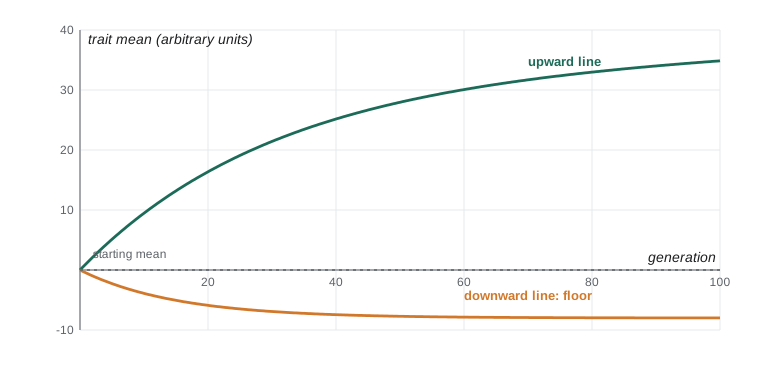
How far can selection push a trait? The Illinois long-term selection experiment on maize began in 1896 and is the longest-running selection experiment in plants. Lines selected for high and low kernel oil and protein content have diverged dramatically over more than 120 generations: oil in the high line rose from about 5 per cent to over 20 per cent, while the low line fell close to zero, which is a physiological floor. Remarkably, the high line has continued to respond long after the original variation might have been expected to run out. Similar continued responses are seen in mice selected for body size or wheel running, and in poultry and dairy cattle.
import numpy as np
rng = np.random.default_rng(3215)
# Polygenic trait: 200 additive loci with small effects; truncation selection of the top 20%
L, N, gens = 200, 500, 100
effects = rng.exponential(0.1, L)
G = rng.binomial(2, 0.5, (N, L))                       # genotypes (0, 1, 2 copies of the '+' allele)
sd_e = (G @ effects).std()                             # environmental SD set so initial h2 is about 0.5
means, h2s = [], []
for t in range(gens):
    g = G @ effects
    z = g + rng.normal(0, sd_e, N)
    means.append(z.mean()); h2s.append(g.var()/z.var())
    parents = np.argsort(z)[-N//5:]                     # top 20%
    mums, dads = rng.choice(parents, N), rng.choice(parents, N)
    G = rng.binomial(1, G[mums]/2) + rng.binomial(1, G[dads]/2)   # each parent passes one allele per locus
    G = G + (rng.random((N, L)) < 1e-4) * (G < 2) * 1   # rare new '+' mutations
for t in (0, 10, 25, 50, 99):
print(f"gen {t:3d}: mean {means[t]-means[0]:6.2f} above start, h2 = {h2s[t]:.2f}")gen 0: mean 0.00 above start, h2 = 0.46 gen 10: mean 11.07 above start, h2 = 0.36 gen 25: mean 17.31 above start, h2 = 0.09 gen 50: mean 19.95 above start, h2 = 0.02 gen 99: mean 20.64 above start, h2 = 0.00
In the simulation, the trait mean rises rapidly at first and then more slowly as favourable alleles approach fixation, and heritability falls toward zero within about 50 generations; the rare new mutations in this small model add too little variation to keep the response going. In real long-term experiments, the response often lasts longer than simple models predict, because traits are influenced by very many loci, new mutations add variation each generation and some alleles have effects that only become visible once others are fixed. Eventually, responses usually slow or stop, sometimes because of opposing natural selection: chickens selected for very rapid growth develop leg and heart problems, and mice selected for large size become less fertile.
Polygenic architecture
Genome-wide association studies (GWAS), which scan hundreds of thousands to millions of genetic variants in large samples, have revealed that most complex traits are extremely polygenic. Height in humans is influenced by thousands of variants, each with a tiny effect. A 2022 study of about 5.4 million people identified over 12,000 independent variants associated with height, which together explained around 40 to 45 per cent of variation in people of European ancestry but considerably less in other groups, largely because most study participants have been of European ancestry. Some researchers have even proposed an omnigenic model, in which nearly every gene expressed in relevant tissues has some small effect on a trait through interconnected regulatory networks.
Polygenic architecture changes how adaptation proceeds. When a trait is influenced by many loci of small effect, a shift in the optimum can be reached by small frequency changes at many loci rather than a sweep of one allele to fixation. Such polygenic adaptation leaves subtle signals in the genome. Early claims of strong polygenic selection on height across European populations were later found to be partly caused by subtle population structure in the GWAS data, a cautionary example showing how difficult these analyses are. Polygenic scores, which add up the estimated effects of many variants for an individual, are used in research and are being explored in medicine, but their predictive power is modest for most traits and is lower in groups underrepresented in the original studies.
Common mistakes
MistakeA heritability of 0.6 means 60 per cent of a person’s trait is caused by genes.
InsteadIt means 60 per cent of the variation among individuals in that population and environment is additive genetic.
MistakeHigh heritability means the trait cannot be changed by the environment.
InsteadHeritability says nothing about how environments change the trait; height is highly heritable yet rose greatly with better nutrition.
MistakeHigh heritability within groups explains differences between groups.
InsteadDifferences between groups can be entirely environmental even when heritability within each group is high.
MistakeSelection on one trait affects only that trait.
InsteadGenetic correlations cause correlated responses in other traits, sometimes opposite to their own selection.
MistakeSelection always stops quickly because genetic variation runs out.
InsteadPolygenic traits and new mutations can sustain responses for over a hundred generations.
MistakeA polygenic score predicts an individual’s trait accurately.
InsteadMost polygenic scores explain only part of the variation and work less well outside the populations studied.
Summary and key terms
- Phenotypic variance is partitioned into additive, dominance, interaction and environmental components; narrow-sense heritability h² = V_A/V_P drives the response to selection.
- Heritability is specific to a population and environment and does not explain differences between groups.
- Parent–offspring regression on midparent values estimates h²; shared environments can bias estimates.
- The breeder’s equation R = h²S, or R = i h² σ_P, predicts response per generation, and dividing by generation interval gives annual gain.
- Genetic correlations, summarized in the G matrix, produce correlated responses; populations tend to evolve along g_max, the line of least resistance.
- Long-term selection experiments, such as the Illinois maize lines since 1896, show sustained responses that eventually meet physiological or fitness limits.
- GWAS show most complex traits are highly polygenic; polygenic adaptation and polygenic scores are powerful but easily misinterpreted.
- quantitative trait
- A trait that varies continuously and is influenced by many genes and the environment.
- additive genetic variance
- Variance due to the average effects of alleles, which determines resemblance between relatives.
- narrow-sense heritability
- The proportion of phenotypic variance that is additive genetic, h² = V_A/V_P.
- breeder’s equation
- R = h²S, predicting the response to selection.
- selection intensity
- The selection differential expressed in phenotypic standard deviations.
- pleiotropy
- The effect of one gene on several traits.
- genetic correlation
- The correlation between the additive genetic effects on two traits.
- G matrix
- The matrix of additive genetic variances and covariances among traits.
- genome-wide association study
- A study that tests many genetic variants for association with a trait.
- polygenic score
- A sum of estimated effects of many variants, used to estimate genetic predisposition.
Practice problems
Work each problem on paper first, then reveal the answer to check.
V_A = 30, V_D = 10, V_E = 60. What are H² and h²?
Show answer
H² = 40/100 = 0.4; h² = 30/100 = 0.3.
Offspring regressed on one parent give a slope of 0.25. Estimate h².
Show answer
h² ≈ 2 × 0.25 = 0.5.
A trait has h² = 0.4 and S = 5 units. What is the predicted response?
Show answer
R = 0.4 × 5 = 2 units.
With i = 1.4, h² = 0.3, σ_P = 10 and a generation interval of 2 years, what is the annual gain?
Show answer
1.4 × 0.3 × 10 / 2 = 2.1 units per year.
Why can heritability fall when an environment becomes more variable?
Show answer
Environmental variance increases, so the additive share of total variance decreases.
How can a trait evolve opposite to the direction of its own selection?
Show answer
If it is genetically correlated with another trait under stronger selection.
What is g_max?
Show answer
The direction of greatest additive genetic variance, along which populations evolve most easily.
Why did selection for very rapid growth in chickens eventually cause problems?
Show answer
Correlated effects on legs and heart opposed by natural selection.
Give one reason polygenic scores are less accurate in some populations.
Show answer
Most GWAS participants have been of European ancestry, so effect estimates and linkage patterns transfer poorly.
What was learned when claims of polygenic selection on height were re-examined?
Show answer
Part of the signal came from uncorrected population structure in the GWAS data.
Lesson quiz · 5 questions
Score 60% or more to complete this lesson.
Create a free account to save your progress, take quizzes and earn a certificate.