
BIOL-108 · Lesson 12 of 12 · 27 min
Ecology basics and capstone: biodiversity, evolution and conservation
Evolution explains where the diversity of life came from; ecology explains how organisms interact with each other and their environments today. The two are tightly linked: ecological interactions are the source of natural selection, and evolutionary history shapes which species live where. This final lesson introduces the basic ideas of ecology, from populations to ecosystems, and then brings the course together in a capstone: analysing an invented biodiversity survey and placing it in the context of conservation law and practice. BIOL-208 (Principles of Ecology), BIOL-367 (Conservation Biology) and BIOL-440 (Boreal and Northern Ecology) build on this lesson.
Levels of ecology
Ecology is studied at nested levels. A population is the members of one species in an area. A community is all the populations of different species living and interacting in an area. An ecosystem is the community together with its physical environment: soil, water, climate and nutrients. A biome is a major type of ecosystem defined by climate and dominant vegetation, such as tundra, boreal forest, temperate deciduous forest, grassland or desert. The biosphere is all life on Earth.
| Biome | Climate | Dominant vegetation | North American example |
|---|---|---|---|
| Arctic tundra | Very cold; short summers; permafrost | Mosses, lichens, sedges, dwarf shrubs | Nunavut, northern Yukon and Alaska |
| Boreal forest (taiga) | Long cold winters; short warm summers | Spruce, fir, pine, larch, birch, aspen | From Yukon and Alaska to Newfoundland and Labrador |
| Temperate deciduous forest | Warm summers, cold winters, rain all year | Maple, oak, beech, hickory | Southern Ontario and Quebec; the eastern United States |
| Temperate grassland | Hot summers, cold winters, moderate rain, periodic drought and fire | Grasses and wildflowers | The Prairies of Alberta, Saskatchewan and Manitoba; the Great Plains |
| Temperate rainforest | Mild, very wet | Giant conifers such as western red cedar and Sitka spruce | Coastal British Columbia, Washington and Oregon; Great Bear Rainforest |
| Desert | Very dry | Cacti, shrubs, drought-adapted annuals | The Sonoran and Mojave deserts; a small arid area near Osoyoos, British Columbia |
Population growth
Populations grow when births and immigration exceed deaths and emigration. With unlimited resources, a population grows exponentially, at a rate proportional to its size: \(\frac{dN}{dt} = rN\), where \(r\) is the per-capita growth rate. Exponential growth cannot last, because resources run out. Populations then tend toward the carrying capacity, \(K\), the largest population the environment can sustain. The logistic model captures this slowing:
The fraction \((K - N)/K\) is the share of the carrying capacity still unused. In words: growth is fast when the population is small relative to \(K\), and slows to zero as the population approaches \(K\).
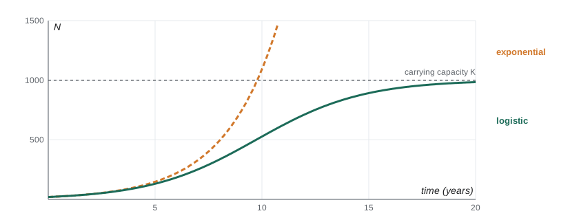
# Exponential versus logistic growth, stepped one year at a time
r, K = 0.4, 1000.0
n_exp = n_log = 20.0
print("year  exponential  logistic")
for year in range(0, 21, 4):
    print(f"{year:4d}  {n_exp:11,.0f}  {n_log:8,.0f}")
    for _ in range(4):
        n_exp += r * n_exp
n_log += r * n_log * (1 - n_log / K)year exponential logistic 0 20 20 4 77 74 8 295 245 12 1,134 603 16 4,356 902 20 16,734 985
Species differ in their life-history strategies. Some, called r-selected, produce many small offspring with little care and boom in unstable environments: mosquitoes, dandelions, mice. Others, called K-selected, produce few large offspring with much care and live near carrying capacity: elephants, whales, oaks, humans. Most species fall between these extremes. K-selected species recover slowly from losses, which is why large, slow-breeding animals such as whales, caribou and sea turtles are often the most vulnerable to overharvest.
Interactions between species
Species interact in several ways, classified by whether each partner gains (+), loses (−) or is unaffected (0).
| Interaction | Effect on each species | Example |
|---|---|---|
| Competition | − / − | Lynx and coyotes competing for snowshoe hares |
| Predation | + / − | Wolves hunting moose; owls hunting mice |
| Herbivory | + / − | Moose browsing willows; caterpillars eating leaves |
| Parasitism | + / − | Winter ticks on moose; tapeworms in wolves |
| Mutualism | + / + | Mycorrhizal fungi and plant roots; bees and flowers |
| Commensalism | + / 0 | Lichens growing on tree bark; barnacles on whales |
Predator–prey relationships can produce cycles. The classic case is the snowshoe hare and the Canada lynx: records of pelts bought by the Hudson's Bay Company over nearly two centuries show both populations rising and falling on a cycle of about ten years, with lynx peaks lagging behind hare peaks. The Lotka–Volterra equations, developed in the 1920s, model this: prey grow on their own but are eaten in proportion to encounters with predators; predators grow by eating prey and die at a constant rate.
# Lotka-Volterra predator-prey model, Euler steps (illustrative parameters)
a, b = 1.0, 0.02      # hare growth rate; predation rate per encounter
c, d = 0.01, 0.8      # lynx growth per hare eaten; lynx death rate
hares, lynx = 60.0, 20.0
dt = 0.01
peaks = []
prev_h, rising = hares, True
for step in range(1, 3001):
    dh = (a * hares - b * hares * lynx) * dt
    dl = (c * hares * lynx - d * lynx) * dt
    hares, lynx = hares + dh, lynx + dl
    if rising and hares < prev_h:
        peaks.append(round(step * dt, 1))
    rising = hares >= prev_h
    prev_h = hares
    if step % 500 == 0:
        print(f"t = {step*dt:4.1f}: hares {hares:6.1f}, lynx {lynx:5.1f}")
print("hare peaks at times:", peaks)t = 5.0: hares 26.7, lynx 60.4 t = 10.0: hares 179.4, lynx 62.5 t = 15.0: hares 57.0, lynx 19.0 t = 20.0: hares 25.0, lynx 62.7 t = 25.0: hares 191.3, lynx 55.1 t = 30.0: hares 49.8, lynx 18.6 hare peaks at times: [2.3, 9.8, 17.4, 24.9]
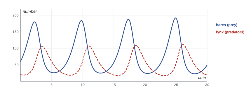
The model is far simpler than reality. Real hare cycles also depend on food plants, stress hormones in hares and other predators such as owls and coyotes, and studies in Yukon's Kluane region showed that food and predation together drive the cycle. Simple models are still useful because they reveal the core mechanism: delayed feedback between predator and prey.
Energy and nutrients in ecosystems
Energy flows through ecosystems in one direction, entering as sunlight captured by producers (plants, algae and cyanobacteria) and passing to primary consumers (herbivores), secondary consumers (carnivores) and decomposers. At each step, most energy is lost as heat through respiration; on average only about 10 per cent passes to the next level. That is why food chains rarely have more than four or five links, and why there are far fewer wolves than moose and far fewer moose than plants.
Nutrients, by contrast, cycle. Carbon is fixed by photosynthesis and released by respiration, decomposition and burning. Nitrogen gas, abundant in air but unusable by most organisms, is fixed by bacteria (lesson 7), taken up by plants, passed through food webs and returned to the air by denitrifying bacteria. Phosphorus cycles mostly through rocks, soils and water. Human activity has greatly altered these cycles: burning fossil fuels adds carbon dioxide to the atmosphere, and fertilizer runoff overloads lakes with nitrogen and phosphorus, fuelling algal blooms.
Some species have effects far out of proportion to their abundance. These keystone species include sea otters, which eat sea urchins and so protect kelp forests along the Pacific coast; beavers, which create wetlands that support many other species; and wolves, whose return to Yellowstone National Park in 1995 changed how elk used the landscape, though the size of the effects on vegetation is still debated.
Measuring biodiversity
Biodiversity includes genetic diversity within species, species diversity and ecosystem diversity. Species diversity has two parts: richness, the number of species, and evenness, how equally individuals are spread among them. Two indices combine both. Simpson's index gives the probability that two individuals picked at random belong to different species: \(D = 1 - \sum p_i^2\). Shannon's index, \(H = -\sum p_i \ln p_i\), comes from information theory. In both, \(p_i\) is the proportion of individuals belonging to species \(i\).
Capstone: an invented biodiversity survey
The capstone brings together ideas from the whole course. Imagine a field team surveys birds along standardized routes in two habitats near a boreal town: an intact older forest and a forest regenerating after logging 15 years ago. The counts below are invented for teaching, but the methods are those used in real surveys.
import math
# Invented bird counts from equal survey effort in two habitats
old = {"boreal chickadee": 22, "red-breasted nuthatch": 18, "brown creeper": 12, "golden-crowned kinglet": 25,
       "black-backed woodpecker": 6, "Canada jay": 9, "bay-breasted warbler": 11, "white-winged crossbill": 14}
regen = {"white-throated sparrow": 48, "chestnut-sided warbler": 20, "American robin": 15,
         "dark-eyed junco": 12, "Canada jay": 4, "golden-crowned kinglet": 3}

def indices(counts):
    n = sum(counts.values())
    p = [c / n for c in counts.values()]
    simpson = 1 - sum(x * x for x in p)
    shannon = -sum(x * math.log(x) for x in p)
    evenness = shannon / math.log(len(p))
    return n, len(p), simpson, shannon, evenness

for name, counts in (("older forest", old), ("regenerating", regen)):
    n, s, d, h, e = indices(counts)
    print(f"{name:<13} birds {n:3d}, species {s}, Simpson {d:.3f}, Shannon {h:.3f}, evenness {e:.2f}")
shared = set(old) & set(regen)
print("species shared:", sorted(shared))older forest birds 117, species 8, Simpson 0.853, Shannon 1.991, evenness 0.96 regenerating birds 102, species 6, Simpson 0.702, Shannon 1.439, evenness 0.80 species shared: ['Canada jay', 'golden-crowned kinglet']
The older forest has more species and a more even community, so both indices are higher; the regenerating stand is dominated by one species, the white-throated sparrow, typical of young, shrubby habitat. But the regenerating stand is not worthless: it supports species, such as chestnut-sided warblers, that the older forest lacks. A landscape with a mix of habitat ages supports more species overall than either alone, an idea ecologists call beta diversity, the turnover of species between habitats.
Next, the team estimates the population of a species of concern, using mark–recapture. In a first session they capture, band and release a number of birds; later they capture a second sample and count how many are already banded. If marked birds mix randomly, the proportion marked in the second sample estimates the proportion marked in the whole population, giving the Lincoln–Petersen estimate \(N \approx \frac{M \times C}{R}\), where \(M\) is the number marked, \(C\) the number caught in the second session and \(R\) the number of those already marked.
import numpy as np
# Lincoln-Petersen estimate, checked against a simulated population of known size
rng = np.random.default_rng(12)
true_N = 400
M, C = 60, 80
estimates = []
for trial in range(1000):
    marked = np.zeros(true_N, dtype=bool)
    marked[rng.choice(true_N, M, replace=False)] = True
    second = rng.choice(true_N, C, replace=False)
    R = marked[second].sum()
    if R > 0:
        estimates.append((M + 1) * (C + 1) / (R + 1) - 1)   # Chapman's bias-corrected version
est = np.array(estimates)
print(f"one field result: M = 60, C = 80, R = 12 -> N = {60 * 80 / 12:.0f}")
print(f"simulation: mean estimate {est.mean():.0f}, 95% of estimates between "
f"{np.percentile(est, 2.5):.0f} and {np.percentile(est, 97.5):.0f} (true N = {true_N})")one field result: M = 60, C = 80, R = 12 -> N = 400 simulation: mean estimate 398, 95% of estimates between 273 and 617 (true N = 400)
The simulation shows that a single mark–recapture study can easily be off by a quarter or more, so real studies repeat sessions and report confidence intervals. Finally, the team asks how much habitat must be protected. The species–area relationship, one of ecology's oldest patterns, says that the number of species \(S\) found in an area \(A\) grows as \(S = cA^z\), with \(z\) typically between about 0.15 and 0.35. It implies that losing habitat loses species, though not in direct proportion.
# Species-area relationship S = c * A^z: expected species remaining after habitat loss
z = 0.25
for remaining in (1.0, 0.5, 0.25, 0.10):
    fraction_species = remaining ** z
print(f"{remaining:5.0%} of habitat left -> about {fraction_species:5.1%} of species expected to persist long term")100% of habitat left -> about 100.0% of species expected to persist long term 50% of habitat left -> about 84.1% of species expected to persist long term 25% of habitat left -> about 70.7% of species expected to persist long term 10% of habitat left -> about 56.2% of species expected to persist long term
Losing half the habitat is expected eventually to cost about 16 per cent of species, and losing 90 per cent to cost about 44 per cent. The losses often arrive with a delay, called an extinction debt, as small isolated populations dwindle through drift, inbreeding (lesson 3) and chance events. Keeping habitat connected, so that gene flow and recolonization can continue, is therefore as important as its total area.
Conservation law and species at risk
Both countries protect threatened species by law, with independent scientific bodies assessing status and governments deciding on legal listing and protection.
In Canada, the Species at Risk Act (SARA, 2002) protects listed wildlife species. The independent Committee on the Status of Endangered Wildlife in Canada (COSEWIC) assesses species as extinct, extirpated, endangered, threatened or of special concern, and the federal government decides whether to add them to Schedule 1 of the Act. Listing triggers prohibitions on killing or harming individuals and their residences, and requires recovery strategies that identify critical habitat. The Act applies directly on federal lands and to aquatic species and migratory birds; elsewhere, provinces and territories have the main responsibility, and the federal minister can recommend an emergency order when a species faces imminent threats. The monarch butterfly was listed as endangered under SARA in December 2023. Woodland caribou are listed in several populations, with boreal caribou threatened; in 2024 the federal environment minister formed the opinion that boreal caribou in Quebec face imminent threats, but in a statement published on 30 June 2026 the government chose to pursue a collaborative approach with Quebec and First Nations rather than an emergency order at that time.
Conservation increasingly draws on Indigenous knowledge alongside Western science. Indigenous peoples have observed and managed ecosystems for thousands of years, and their knowledge of species, seasons and landscapes often extends further back in time than scientific records. In Canada, the Mi'kmaw concept of Etuaptmumk, or Two-Eyed Seeing, articulated by Elder Albert Marshall, describes learning to see with the strengths of Indigenous knowledge in one eye and Western knowledge in the other, and Indigenous Guardians programs employ community members to monitor lands and waters. In the United States, many tribal natural resource departments manage fisheries and wildlife, and federal agencies have issued guidance on including Indigenous knowledge in decisions. Respectful collaboration means communities decide how their knowledge is shared and used.
Bringing it together
The capstone shows how the course's ideas connect. The bird species in the survey are products of natural selection (lesson 2) and speciation (lesson 4) over millions of years, related as branches of a tree (lesson 6). Their populations are shaped by competition, predation and habitat. Their persistence depends on keeping populations large and connected enough to resist drift and inbreeding (lesson 3). And the law and ethics of conservation decide what is protected. Evolution is not just the history of life: it is a process continuing around us, in antibiotic-resistant bacteria, changing flowering times, and the species we are trying to save.
Common mistakes
MistakePopulations grow without limit if left alone.
InsteadGrowth slows as resources become limiting; populations approach a carrying capacity.
MistakeEnergy cycles through ecosystems like nutrients.
InsteadEnergy flows one way and is lost as heat at each step; nutrients such as carbon and nitrogen cycle.
MistakeA habitat with more individuals always has more biodiversity.
InsteadDiversity depends on species richness and evenness, not just total abundance.
MistakeHalving habitat halves the number of species immediately.
InsteadThe species–area relationship predicts smaller proportional losses, often delayed as an extinction debt.
MistakeMark–recapture gives an exact population count.
InsteadIt gives an estimate with uncertainty that depends on sample sizes and on assumptions such as random mixing.
Summary and key terms
- Ecology studies populations, communities, ecosystems, biomes and the biosphere.
- Exponential growth (dN/dt = rN) gives way to logistic growth limited by carrying capacity K.
- Species interact through competition, predation, herbivory, parasitism, mutualism and commensalism; predator–prey interactions can cycle.
- Energy flows one way with about 10 per cent passing between trophic levels; nutrients cycle.
- Simpson and Shannon indices measure diversity combining richness and evenness.
- Mark–recapture estimates population size; the species–area relationship predicts species loss from habitat loss.
- Canada’s SARA and the US ESA protect species at risk; Indigenous knowledge increasingly guides conservation.
- population
- The members of one species living in an area.
- community
- All the populations of different species living and interacting in an area.
- ecosystem
- A community together with its physical environment.
- carrying capacity
- The largest population an environment can sustain over time.
- logistic growth
- Population growth that slows as it approaches carrying capacity.
- keystone species
- A species with an effect on its community far larger than its abundance suggests.
- trophic level
- A position in a food chain, such as producer, herbivore or carnivore.
- species richness
- The number of species in a community.
- Simpson’s diversity index
- The probability that two randomly chosen individuals belong to different species.
- species–area relationship
- The pattern that species number increases with area as S = cA^z.
Practice problems
Work each problem on paper first, then reveal the answer to check.
Arrange in order from smallest to largest: ecosystem, population, biome, community.
Show answer
Population, community, ecosystem, biome.
With r = 0.5 and K = 200, how fast does a population of 100 grow by the logistic model?
Show answer
dN/dt = 0.5 × 100 × (1 − 100/200) = 25 per unit time.
Why do lynx population peaks lag behind hare peaks?
Show answer
Lynx numbers rise only after hares become abundant, and fall after hares decline.
Classify: a fungus helps a plant root absorb phosphorus and receives sugar.
Show answer
Mutualism (+/+).
If producers capture 10,000 kJ, roughly how much reaches secondary consumers?
Show answer
About 100 kJ (10 per cent of 10 per cent).
A community has two species with 50 individuals each. What is Simpson’s index?
Show answer
D = 1 − (0.5² + 0.5²) = 0.5.
M = 40 birds marked, C = 50 caught later, R = 10 marked. Estimate N.
Show answer
N ≈ 40 × 50 / 10 = 200.
With z = 0.25, what fraction of species is expected to persist if 25 per cent of habitat remains?
Show answer
0.25^0.25 ≈ 0.71, about 71 per cent.
What is the role of COSEWIC in Canada?
Show answer
It independently assesses species’ status; the government then decides on listing under SARA.
Why is habitat connectivity important for species at risk?
Show answer
It allows gene flow and recolonization, countering drift, inbreeding and local extinction.
Lesson quiz · 5 questions
Score 60% or more to complete this lesson.
Create a free account to save your progress, take quizzes and earn a certificate.