
BAS-330 · Lesson 12 of 12 · 25 min
An energy retrofit through the control system
▶ Video coming soon A video version of this lesson is on the way.
On Friday, November 13, Prakash re-seated the coupling on room 108's reheat valve before 9:00, and by noon the box's discharge air was within a degree of the supply air for the first time in weeks. At about 4:30 that afternoon, back at the office, Declan put his draft of the Ninefield Tower retro-commissioning proposal on the table and asked Callie to check it with him, line by line. The proposal would go to Ilona Vescovi in early December, the work would be done in the spring of 2027, and the year after that would show whether it had worked. "Everything you have learned on Thursdays is in here," he said. "If any of it is wrong, now is when we find out."
This lesson follows the proposal from the data to the measures, the estimates, the M&V plan and the risks, as a worked example of an energy retrofit carried out mostly through the control system.
Step 1: what the data said
Declan's starting point was the analysis from the autumn: the bills, PM-1's 15-minute data since August, the trends Quillon had set up, and what Callie, Prakash and Sophie had found on site.
| Finding | Evidence | Lesson |
|---|---|---|
| Site EUI 216 ekWh/m² (68.7 kBtu/ft²), ENERGY STAR score 52 | 2025 bills, Portfolio Manager | Lessons 1 and 10 |
| Night and weekend base load about 150 kW, 30 in 100 of electricity | PM-1 15-minute data | Lesson 1 |
| Monthly peaks set by coincident starts at 6:00 (820 kW July, 760 kW January) | Bills and PM-1 data | Lessons 2 and 6 |
| All equipment on a fixed 6:00 start for 7:00 occupancy | Schedules on the front end | Lesson 4 |
| Fixed duct static setpoints on both penthouse air handlers | Programs and trends | Lesson 5 |
| One air handler's supply air setpoint lowered to 10 °C (50 °F) | Program and trends | Lesson 5 |
| Secondary pumps near 52 Hz all day; three-way valves; low delta-T 3.5 K (6.3 °F) | Trends, valve survey | Lesson 5 |
| Chilled water meter reading about 28 in 100 low | Portable meter comparison in September | Lesson 3 |
| Outdoor air dampers on one air handler open during warm-up | Trends of damper command and mixed air temperature | Lesson 4 |
| Occupancy sensors on every floor from the 2019 lighting controls, not used by HVAC | Lighting gateway point list | Lesson 4 |
Callie noticed that almost every finding had been made by someone looking at data that already existed. Only two, the low chilled water meter and the warm-up dampers, had needed a site visit to confirm.
Step 2: the base load
The base load was the largest opportunity, so Declan had spent a night in the building in October with the front end on a laptop, as he had described in the first session. He had found that the base load was made up of the elevators, emergency lighting, two tenants' server closets with their own cooling, the garage and toilet exhaust fans, the podium's retail refrigeration, and a handful of things that should not have been on: two rooftop unit supply fans running continuously because their old controllers had lost their schedules, a corridor lighting zone overridden on, and perimeter fan-powered box fans running all night on three floors because their unoccupied mode had been programmed wrongly in 1998.
Worked problem
The base load measure
Declan estimated that fixing the schedules and modes would bring the average base from 150 kW to about 125 kW, more conservatively than the 110 kW used as an illustration in lesson 1. What is the annual saving?
Show solution
- Unoccupied hours: 108 a week × 52 = 5,616 h.
- Saving: (150 − 125) × 5,616 = 140,400 kWh.
Answer: About 140,400 kWh a year, the largest single measure in the proposal, for the cost of a few days of programming and checking. The new rooftop unit controllers going in during December would fix the first part.
Step 3: the measures
Each measure in the proposal had a description, the sequence change, an estimate with its method, and the M&V option. Declan summarized them in one table.
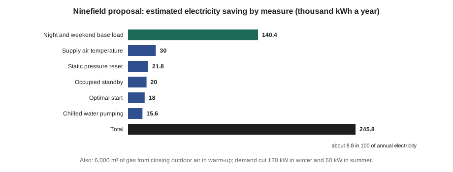
| Measure | Control change | Electricity saved | Estimate method |
|---|---|---|---|
| 1. Night and weekend base load | Fix schedules, unoccupied modes, overrides | 140,400 kWh | 25 kW × unoccupied hours |
| 2. Duct static pressure reset | Trim and respond on both penthouse air handlers | 21,800 kWh | Fan power at reduced pressure (lesson 5) |
| 3. Supply air temperature | Restore 13 °C (55 °F) and add trim and respond reset | 30,000 kWh | Reheat and cooling avoided |
| 4. Chilled water pumping | Two-way valves, remote DP sensor, DP reset | 15,600 kWh | Pump kW at reduced speed, derated from cube law |
| 5. Optimal start | Adaptive start with earliest and latest limits, staggered | 18,000 kWh | Run hours saved on mild mornings |
| 6. Occupied standby | Use lighting occupancy sensors for HVAC setback by zone | 20,000 kWh | Setback hours from lighting sensor data |
| 7. Outdoor air in warm-up | Close dampers until occupancy; repair actuator | Gas 6,000 m³ (2,120 therms) | Outdoor air heating hours |
| 8. Demand control | Staggered starts and predictive demand limit | Demand only | 120 kW winter, 60 kW summer |
The total electricity saving was 245,800 kWh, about 8.8 in 100 of the 2,800,000 kWh annual use. Declan had not simply added up the measures' best cases. He had deliberately estimated each one conservatively, and noted that some interact: the static pressure reset saves a little less once occupied standby has reduced airflow to empty zones, and the supply air temperature reset slightly increases fan airflow. For a package of interacting measures, the total from whole-building M&V is the number that counts, and individual estimates are for planning.
Two items were in the proposal without savings attached: the magnetic chilled water flow meter with matched temperature sensors, which would let the plant's efficiency be measured properly for the first time, and tagging the 1998 tower points so that the fault detection platform could be added later.
Step 4: what it is worth
Worked problem
The annual saving in money
Using sample rates of 0.13 dollars per kWh for energy and its per-kWh charges, 0.45 dollars per m³ for gas, and 11.50 dollars per kW per month for demand, value the measures. The demand reductions are 120 kW for four winter months and 60 kW for five summer months.
Show solution
- Electricity: 245,800 × 0.13 = 31,954 dollars.
- Gas: 6,000 × 0.45 = 2,700 dollars.
- Demand, winter: 120 × 11.50 × 4 = 5,520 dollars; summer: 60 × 11.50 × 5 = 3,450 dollars.
- Total: 31,954 + 2,700 + 5,520 + 3,450 = 43,624 dollars a year.
Answer: About 43,600 dollars a year at the sample rates. The proposal would use the rates on Ninefield's current tariff and state the date of the rates used.
Worked problem
Simple payback
Quillon's price for the work, including the two-way valves, the flow meter, programming, tagging, testing and the first year of M&V, was 124,000 dollars. What is the simple payback?
Show solution
- Payback = 124,000 ÷ 43,624 = 2.8 years.
Answer: About 2.8 years, which Ilona's owners would consider attractive. Simple payback ignores the time value of money and the measures' life; for a decision, an owner may also want the net present value over the life of the measures.
Callie added one line to the summary that Declan liked: emissions. At the sample factors from lesson 11, the electricity saving avoids about 14.7 t of CO₂e a year and the gas saving about 11.4 t, about 26 t in all, which Ilona could report alongside the Portfolio Manager results.
Step 5: the M&V plan
Declan's M&V section followed the outline from lesson 9.
| Item | Plan |
|---|---|
| Whole-building savings | Option C on electricity, using a model of 15-minute utility interval data against hourly outdoor temperature, separate for occupied and unoccupied hours; and on gas, using monthly bills against heating degree-days |
| Measure-level checks | Option B on fan and pump drive kW for measures 2 and 4; Option A for optimal start using run hours |
| Baseline period | September 2025 to August 2026, with the building's conditions recorded: occupancy by floor, hours, tenants, setpoints |
| Installation period | Spring 2027, excluded from both periods |
| Reporting period | Twelve months starting the month after the work is accepted |
| Adjustments | Weather in the model; any non-routine adjustment above 1 in 100 of the baseline agreed in writing with Ilona |
| Pricing | Savings valued at the tariff in force during the reporting period |
| Reporting | Monthly one-page report and call; annual M&V report at the end of the reporting year |
Callie checked the statistics on the gas baseline herself from the numbers in lesson 9: R² of 0.99 and a CV(RMSE) of 7.7 in 100, within the commonly cited Guideline 14 limit for monthly models. The electricity model would be built from interval data during the winter, before the work started, so that its accuracy could be stated in the final proposal.
Step 6: the sequences and the testing
Every measure was a sequence change, and every sequence change needed testing. Sophie had already drafted most of the sequences in BAS-230's sessions: the static pressure and supply air resets, the hydronic DP reset with its remote sensor and fallback, the restart inhibit from BAS-220, the occupied standby rules. The proposal referred to the sequence document rather than repeating it, and added a testing section based on BAS-220's test plan approach: each sequence tested on the bench where possible, then functionally in the building, with trends to show it working before and after.
Functional test record (extract), measure 2: duct static pressure reset
  Test 1  All zones satisfied, requests = 0
          Expect: setpoint trims 12 Pa every 2 min down to SPmin
  Test 2  Force 4 zones to request (I = 2)
          Expect: setpoint rises 30 Pa per step, limited to 32 Pa
  Test 3  Remove requests
          Expect: setpoint trims back; no hunting of fan speed
  Test 4  Fail the duct static sensor
          Expect: fan holds last speed, alarm, operator notified
  Trend for 7 days after acceptance:
          setpoint, fan speed, fan kW, requests, worst zone damper position
Testing the rogue zones came first. The static pressure reset would only work if no box requested constantly, so the proposal included a week of trending zone requests before the reset was enabled, and a budget to fix the boxes that requested all the time. Callie recognized room 108's lesson: fix the zone, not the setpoint.
Step 7: risks and how to handle them
| Risk | Effect | How the proposal handles it |
|---|---|---|
| Rogue zones defeat the resets | Little fan or pump saving | Trend requests first; budget to fix the worst boxes |
| Tenants complain after setback or standby changes | Settings reversed, savings lost | Tell tenants in advance; comfort KPI on the monthly report; after-hours request timers |
| The hot zone behind the lowered supply air setpoint returns | Pressure to lower it again | Find and fix the zone before raising the setpoint |
| Changes in occupancy during the reporting year | Savings hidden or exaggerated | Record baseline conditions; non-routine adjustments agreed in writing |
| Savings fade after the first year | Lost savings | Monthly KPIs and audit trail review under the service contract |
| Chiller plant interactions with the valve conversion | Unexpected flow or delta-T behaviour | Coordinate with Tarrant Chiller Service; test at low load in spring |
"Most of these are about people, not equipment," Callie said. Declan agreed. A controls retrofit saves energy in the programs, but it keeps saving only if the people in the building understand what changed and why, and if someone keeps looking at the data. That was why the proposal ended with the monthly report, the training for Ilona's building operator, and the service visits, not with the payback.
Step 8: the timeline
| When | What |
|---|---|
| Friday, November 13, 2026 | Draft reviewed by Declan and Callie |
| Early December 2026 | Proposal sent to Ilona; rooftop units 2 to 4 replaced under the existing order |
| Winter 2026 to 2027 | Electricity baseline model built; zone requests trended; rogue boxes listed |
| Spring 2027 | Retro-commissioning work, sequences tested and accepted |
| Following 12 months | Reporting period, monthly reports, annual M&V report |
As Callie packed up, Declan handed her one more page: the room 108 rule, written up for the AHU-2 replacement proposal that would go to Gus in early December, with her name in the credits. "The rule you wrote on Thursday," he said, "is now part of two proposals. That is how energy work goes. You find one leaking valve, and then you go looking for all of them."
Bringing the course together
| Lesson | Where it appears in the proposal |
|---|---|
| 1. How buildings use energy | EUI, base load and load profile |
| 2. Bills and demand charges | Valuing energy, gas and demand separately |
| 3. Metering | PM-1, drive kW, the new chilled water meter |
| 4. Scheduling and optimal start | Measures 1, 5, 6 and 7 |
| 5. Resets | Measures 2, 3 and 4 |
| 6. Demand limiting | Measure 8 |
| 7 and 8. Fault detection and analytics | Tagging, future platform, the room 108 rule |
| 9. M&V | The M&V plan |
| 10. Codes and benchmarking | ENERGY STAR score and reporting |
| 11. Decarbonization | Emissions reporting; heat recovery for the longer term |
Common mistakes
MistakeAdding up best-case savings for each measure.
InsteadEstimate conservatively and remember that measures interact; whole-building M&V gives the real total.
MistakeValuing all savings at one blended price.
InsteadValue energy, gas and demand separately at the current tariff.
MistakeEnabling resets before fixing rogue zones.
InsteadTrend requests first and fix the boxes that request constantly.
MistakeLeaving the M&V plan until after the work.
InsteadAgree the plan before the work starts.
MistakeTreating the payback as the end of the project.
InsteadPlan monthly reporting, training and service so savings persist.
Summary and key terms
- An energy retrofit through the controls starts with data the building already has.
- Night and weekend base load is often the largest and cheapest opportunity.
- Each measure needs a sequence change, an estimate with its method, a test and an M&V option.
- Value electricity, gas and demand separately; show payback and emissions.
- Whole-building M&V with interval data shows the total; measure-level M&V shows each measure.
- Most risks to savings are about people and persistence, not equipment.
- A good proposal ends with reporting, training and service, not with the payback.
- Retro-commissioning
- Commissioning an existing building to restore and improve its operation.
- Measure
- One specific change expected to save energy or cost.
- Interaction
- The effect one measure has on the savings of another.
- Simple payback
- Installed cost divided by annual saving.
- Net present value
- The value today of future savings minus costs, allowing for the time value of money.
- Functional test
- A test showing that a sequence works as specified in the real building.
- Acceptance
- The point at which the owner agrees the work is complete and working.
- Persistence
- The continuation of savings over time.
Practice problems
Work each problem on paper first, then reveal the answer to check.
A measure costs 30,000 dollars and saves 12,000 dollars a year. What is the simple payback?
Show answer
2.5 years.
Base load falls from 140 to 120 kW over 5,616 unoccupied hours. What is the saving?
Show answer
20 × 5,616 = 112,320 kWh.
Why did Declan use whole-building M&V for the package?
Show answer
The measures interact and the total is large enough to see on the main meter.
Why trend zone requests before enabling a reset?
Show answer
To find and fix rogue zones that would hold the setpoint at maximum.
Name two ways the proposal protects savings after the first year.
Show answer
Monthly KPIs and report, audit trail review, operator training, service visits.
Lesson quiz · 5 questions
Score 60% or more to complete this lesson.
Create a free account to save your progress, take quizzes and earn a certificate.