
BAS-330 · Lesson 9 of 12 · 23 min
Measurement and verification of savings
▶ Video coming soon A video version of this lesson is on the way.
Ilona Vescovi had one question about every energy proposal Quillon had ever sent her, and Declan quoted it to Callie: "How will I know it worked?" Savings are the energy a building did not use, which nobody can meter directly. The building cannot be run with and without the retrofit in the same year and the same weather. Measurement and verification, usually shortened to M&V, is the discipline of estimating that missing number fairly enough that an owner, a utility program or a lender will accept it. Declan took Callie through the M&V section of his Ninefield draft.
Savings are a comparison
Savings are always the difference between what the building used and what it would have used without the change, under the same conditions. The second number is the adjusted baseline, and it has to be calculated.
Two periods define the comparison. The baseline period is a representative stretch before the change, usually a full year so that every season is included. The reporting period is the stretch after the change over which savings are claimed. Between them there may be an installation period, which is left out of both.
Simply comparing this year's bill with last year's is not M&V. If the reporting year is colder, a building with genuine savings can appear to use more; if it is milder, a building with none can appear to save. The adjusted baseline takes out the differences that have nothing to do with the change.
The IPMVP options
The International Performance Measurement and Verification Protocol (IPMVP), published by the Efficiency Valuation Organization, is the most widely used framework. It defines four options, which differ in what is measured.
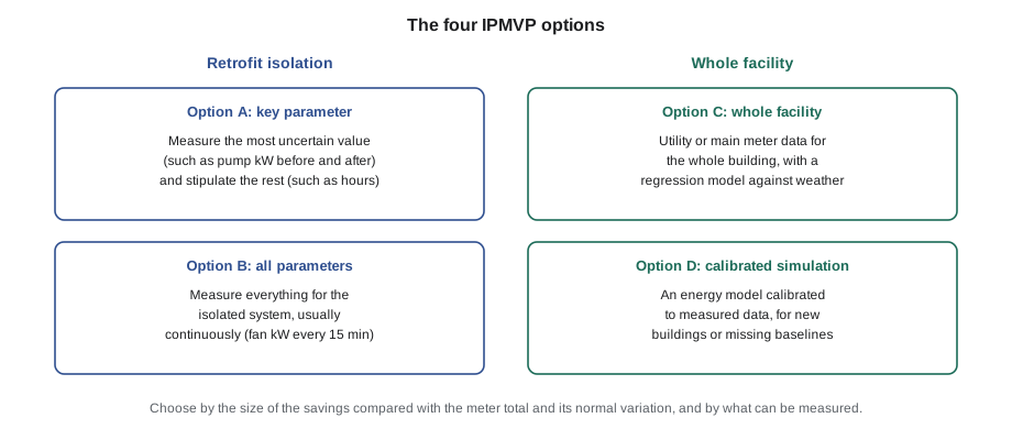
| Option | What is measured | Suits | Ninefield example |
|---|---|---|---|
| A: key parameter | The most uncertain value measured, others estimated and agreed | Simple measures with one key unknown | Pump kW measured before and after; run hours from the schedule |
| B: all parameters | All values for the isolated system, usually continuously | Measures on one system with its own meter | Penthouse air handler fan kW from the drives, every 15 minutes |
| C: whole facility | Main meter or utility bills for the whole building | Savings above roughly 10 in 100 of the meter, or many interacting measures | PM-1 and gas bills, adjusted for weather |
| D: calibrated simulation | An energy model calibrated to measured data | New buildings or where no baseline exists | Not needed |
The choice depends mostly on the size of the expected savings compared with the meter's total and its normal variation. A measure that saves 1 in 100 of a building's electricity is invisible on the main meter, because normal variation is larger than that; it needs Option A or B. A package of measures that saves 10 in 100 or more can be seen on the main meter, and Option C captures all the interactions between measures, including ones nobody predicted.
Declan's plan for Ninefield used both: Option C on PM-1 and the gas bills for the whole retro-commissioning package, which he expected to save around 9 in 100 of the electricity, and Option B on the drive kW readings for the fan and pump resets, so that each of those measures could be shown on its own and tuned if it fell short.
Weather normalization with degree-days
Heating energy depends mostly on how cold it was. A degree-day measures that: for each day, the number of degrees by which the day's average outdoor temperature fell below a base temperature, summed over the period.
The conventional base is 18 °C (65 °F), on the assumption that heat from people, lights and the sun keeps the building warm until the outdoor temperature falls below it. Cooling degree-days are the mirror image for hot weather. Degree-day data for any weather station is published by the national weather service and by many websites, and analytics platforms calculate it from their own weather feeds. A building's true balance point, the temperature below which it actually needs heat, may be quite different from the conventional base, and better models find it from the data.
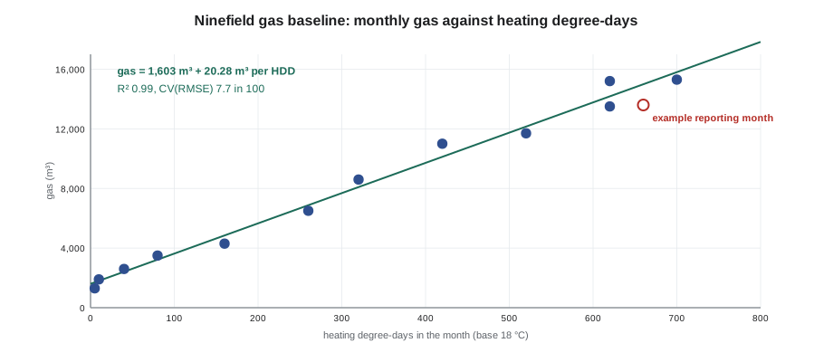
With a year of monthly gas use and the degree-days for each month, a straight line fitted by least-squares regression gives the baseline model: a fixed amount per month for loads that do not depend on weather, such as domestic hot water, plus an amount per degree-day.
| Month | Heating degree-days | Gas used | Model | Difference |
|---|---|---|---|---|
| Jan | 700 | 15,300 m³ | 15,802 m³ | −502 |
| Feb | 620 | 15,200 | 14,179 | +1,021 |
| Mar | 520 | 11,700 | 12,151 | −451 |
| Apr | 320 | 8,600 | 8,094 | +506 |
| May | 160 | 4,300 | 4,848 | −548 |
| Jun | 40 | 2,600 | 2,414 | +186 |
| Jul | 5 | 1,300 | 1,704 | −404 |
| Aug | 10 | 1,900 | 1,806 | +94 |
| Sep | 80 | 3,500 | 3,225 | +275 |
| Oct | 260 | 6,500 | 6,877 | −377 |
| Nov | 420 | 11,000 | 10,122 | +878 |
| Dec | 620 | 13,500 | 14,179 | −679 |
| Total | 3,755 | 95,400 m³ | 95,400 m³ | 0 |
Worked problem
Using the baseline in a future month
After the retro-commissioning work, suppose January 2028 has 660 (1,188) heating degree-days and Ninefield uses 13,600 m³ (4,809 therms) of gas. What are the adjusted baseline and the savings for the month?
Show solution
- Adjusted baseline: 1,603 + 20.28 × 660 = 1,603 + 13,385 = 14,988 m³.
- Savings: 14,988 − 13,600 = 1,388 m³, about 9 in 100 of the adjusted baseline.
Answer: About 1,390 m³ (490 therms) saved in that month. Note that January 2028 was milder than the baseline January, so a raw comparison with January 2026 would have overstated the saving: 15,300 − 13,600 = 1,700 m³ (5,410 − 4,809 = 601 therms).
How good is the model?
A baseline model is a prediction, and it is only as useful as it is accurate. Three statistics are commonly checked.
- The coefficient of determination, R², is the share of the month-to-month variation that the model explains. Ninefield's gas model has R² = 0.99, because gas use is driven almost entirely by heating.
- CV(RMSE), the coefficient of variation of the root mean square error, is the typical size of the model's error as a fraction of average use. Ninefield's is about 7.7 in 100.
- NMBE, the normalized mean bias error, shows whether the model is biased high or low overall. A least-squares fit over its own baseline data has an NMBE of essentially zero.
ASHRAE Guideline 14, a widely used technical companion to the IPMVP, sets limits for calibrated baseline models; for monthly data it is commonly cited as a CV(RMSE) no greater than 15 in 100 and an NMBE within 5 in 100. The deeper test is whether the expected savings are larger than the model's uncertainty. A model with a CV(RMSE) of 7.7 in 100 on monthly data can still show a 9 in 100 saving over a year, because errors in individual months partly cancel over twelve, but it could not reliably show a 2 in 100 saving.
Electricity models and interval data
Electricity at Ninefield depends on weather in both directions: electric perimeter heat in winter and chillers in summer. A monthly model for it uses both heating and cooling degree-days, or a change-point model that finds the temperatures at which heating and cooling begin. With 15-minute data from PM-1, much better models are possible: separate models for occupied and unoccupied hours, using hourly outdoor temperature. Interval models can show savings within weeks, rather than waiting for a full year of bills, and they make night and weekend savings visible directly.
The baseline for Ninefield had a practical limit: PM-1 had only been trended since mid-August 2026, so a full year of interval data would not exist until August 2027, after the spring work. Declan's draft therefore used the utility's 15-minute interval data for the baseline year, downloaded through the utility's portal, and checked it against PM-1 for the months where both existed, as Callie had done for July.
Adjustments
Weather is a routine adjustment: it is expected, measured and built into the model. Other changes are non-routine adjustments, because they are not part of the model and must be handled one at a time.
| Change after the baseline | Effect | Adjustment |
|---|---|---|
| A tenant adds a server room | Electricity rises with no link to the retrofit | Meter or estimate the new load and add it to the adjusted baseline |
| A floor becomes vacant | Use falls with no link to the retrofit | Estimate the effect and subtract it, or exclude the floor |
| Operating hours extended on Saturdays | More hours of operation | Model hours as a variable or adjust by measured kW per hour |
| The 7th-floor fit-out is completed | Different loads and schedule on one floor | Document the change and agree the adjustment with the owner |
| A chiller is replaced under a separate project | Savings that are not the retro-commissioning's | Measure separately and exclude |
The M&V plan should list the conditions of the baseline (occupancy, hours, equipment, setpoints) so that changes can be recognized later. Declan's draft listed them, along with the rule that any adjustment above 1 in 100 of the baseline had to be agreed in writing with Ilona.
Persistence: keeping savings
Savings from controls are easy to lose. A reset disabled during a complaint, a schedule put back to all-day by a new tenant, an override left on: within two or three years, many controls projects have lost much of their savings. That is the strongest argument for keeping M&V running after the first year, and for the monthly report described in lesson 8. If the measured savings drop, the cause is almost always a control change that can be found in the BAS's audit trail and reversed.
Declan's draft proposed a reporting year starting the month after the spring work was accepted, followed by monthly tracking of the same KPIs for as long as Quillon held the service contract.
The M&V plan
Every project that claims savings should have a written M&V plan before work starts. Declan's covered:
- The measures, and the IPMVP option for each.
- The measurement boundary: the whole building for Option C, each system for Option B.
- The baseline period and its data, with the conditions of the building in that period.
- The model and its statistics, and the independent variables: degree-days, occupied hours.
- The reporting period, the meters and intervals, and who collects the data.
- How adjustments will be made, and who agrees them.
- How savings will be priced: at the rates in the baseline year or the reporting year, stated in advance.
- Who prepares the report, when, and what it contains.
"The plan matters more than the math," Declan said. "If we agree the rules before the work, the arguments afterward are short."
Uncertainty, briefly
Every savings figure has an uncertainty, from the model, the meters and the adjustments. The model's share can be estimated from its statistics: a monthly model with a CV(RMSE) of 7.7 in 100 predicts any single month only to within several parts in 100, but over a full year the errors partly cancel and the annual uncertainty is much smaller. A rule of thumb often used is that the expected savings should be at least two or three times the model's annual uncertainty for the result to be meaningful. Guideline 14 gives formulas for the fractional savings uncertainty, and analytics platforms calculate it automatically; the important habit is to report savings with their uncertainty, not as a single exact number.
Stipulated values in Option A
Option A measures the most uncertain value and stipulates the others: they are estimated and agreed in advance, rather than measured. For a pump reset, the key parameter is the pump's power before and after, which is measured; the operating hours might be stipulated from the schedule. Stipulated values must be reasonable and documented, and the owner must agree them, because any error in a stipulated value passes straight into the savings. Declan used Option A only for optimal start, where the run hours could be read from the BAS and the fan and chiller power had been measured.
Worked problem
An Option A estimate
A pump reset reduces measured pump power from 15.0 kW to 9.0 kW. The pump's annual operating hours are stipulated at 2,600 from the cooling season schedule. What are the Option A savings, and what happens if the true hours are 2,400?
Show solution
- Savings with stipulated hours: (15.0 − 9.0) × 2,600 = 15,600 kWh.
- With true hours of 2,400: 6.0 × 2,400 = 14,400 kWh.
Answer: 15,600 kWh is claimed; if the stipulation is 200 hours too high, the claim is 1,200 kWh too high. That is why stipulated values should be conservative and agreed in writing.
Common mistakes
MistakeComparing this year's bill with last year's and calling the difference savings.
InsteadAdjust the baseline for weather and other changes.
MistakeUsing Option C for a measure that saves 1 in 100 of the building's energy.
InsteadUse retrofit isolation, Option A or B, for small savings.
MistakeUsing a baseline period shorter than a full cycle of seasons.
InsteadUse at least 12 months for weather-dependent loads, unless interval models justify less.
MistakeIgnoring a tenant change because it complicates the report.
InsteadRecord it and make a non-routine adjustment agreed with the owner.
MistakeStopping measurement after the first year.
InsteadTrack savings for persistence; most losses are reversible control changes.
Summary and key terms
- Savings are adjusted baseline energy minus reporting period energy, plus or minus adjustments.
- The IPMVP defines Options A and B for retrofit isolation, C for the whole facility and D for calibrated simulation.
- Degree-days measure heating and cooling weather; regression against them gives a baseline model.
- R², CV(RMSE) and NMBE describe a model's accuracy; savings must exceed its uncertainty.
- Interval data allows better models and faster results than monthly bills.
- Routine adjustments are in the model; non-routine adjustments are handled one by one.
- Persistence tracking keeps savings from fading; a written M&V plan comes before the work.
- Measurement and verification (M&V)
- The process of estimating energy savings fairly from measured data.
- Baseline period
- A representative period before a change, used to build the baseline model.
- Reporting period
- The period after a change over which savings are claimed.
- Adjusted baseline
- The energy the building would have used in the reporting period without the change.
- IPMVP
- The International Performance Measurement and Verification Protocol.
- Degree-day
- A measure of how much colder or warmer a day was than a base temperature.
- CV(RMSE)
- The typical model error as a fraction of average use.
- Non-routine adjustment
- An adjustment for a change outside the baseline model, such as a new tenant load.
Practice problems
Work each problem on paper first, then reveal the answer to check.
A day averages 4 °C. How many heating degree-days at base 18 °C?
Show answer
18 − 4 = 14.
Baseline model: 1,603 m³ + 20.28 m³/HDD. Predict a month with 500 HDD.
Show answer
1,603 + 10,140 = 11,743 m³.
That month used 10,900 m³. What are the savings?
Show answer
11,743 − 10,900 = 843 m³.
A measure saves an expected 15,000 kWh in a 2,800,000 kWh building. Which option suits it?
Show answer
Option A or B; 0.5 in 100 is invisible on the main meter.
Name a non-routine adjustment.
Show answer
A new server room, a vacant floor, extended hours, a separate equipment replacement.
Lesson quiz · 5 questions
Score 60% or more to complete this lesson.
Create a free account to save your progress, take quizzes and earn a certificate.