
AERO-440 · Lesson 7 of 12 · 26 min
Solving the Euler equations
The first production question for the group comes from Kenji. The Swift 900 wing must cruise at Mach 0.80 without strong shocks, and the high-speed group has three candidate supercritical sections. A viscous calculation of each at a dozen Mach numbers and lift coefficients would take weeks of computer time. An Euler calculation, inviscid but fully nonlinear and compressible, captures the shock position and strength at a fraction of the cost, and is a sound first screen when the boundary layer is thin and attached. Before trusting an Euler code with the Swift 900, Arjun tests the algorithm on the most famous test case in compressible CFD: the Sod shock tube.
The Euler equations in conservation form
The Euler equations express conservation of mass, momentum and energy for an inviscid, non-heat-conducting gas. In one dimension, in conservation form,
Here \(E = p/(\gamma - 1) + \tfrac12\rho u^{2}\) is the total energy per unit volume for a perfect gas with ratio of specific heats \(\gamma\), 1.4 for air. In three dimensions there are five equations, with fluxes in each coordinate direction. The system is hyperbolic: writing it as \(\mathbf{U}_t + A\,\mathbf{U}_x = 0\), with the flux Jacobian \(A = \partial\mathbf{F}/\partial\mathbf{U}\), the matrix \(A\) has real eigenvalues \(u - c\), \(u\) and \(u + c\), where \(c\) is the speed of sound. These are the speeds of the three families of waves: an acoustic wave travelling upstream relative to the flow, an entropy or contact wave carried with the flow, and an acoustic wave travelling downstream. In three dimensions, two further waves move at speed \(u\), carrying shear.
The eigenvalues are the heart of the numerical problem. In subsonic flow, \(u - c\) is negative while \(u\) and \(u + c\) are positive, so information travels both ways and a single upwind direction does not exist. A scheme must treat each wave family according to the sign of its own speed. This is what the Riemann solvers of lesson 4 and the flux-splitting methods below accomplish.
Upwind schemes for the Euler equations
Flux-vector splitting divides the flux into a part carried by positive waves and a part carried by negative waves, \(\mathbf{F} = \mathbf{F}^{+} + \mathbf{F}^{-}\), and differences each from its upwind side. The Steger-Warming splitting of 1981 does this using the signs of the eigenvalues; it is simple but has a kink at sonic points. Van Leer's splitting, from 1982, uses polynomials in Mach number that are smooth through Mach 1. Flux-vector splitting is robust and was popular in early codes, but it adds dissipation on contact and shear waves that smears boundary layers.
Flux-difference splitting, the Godunov approach, solves a Riemann problem at each face. The Roe solver decomposes the jump into the three waves exactly for the linearized problem, and gives sharp shocks and contacts. The HLL solver of Harten, Lax and van Leer instead assumes that the fastest left- and right-going waves bound a single averaged state, which gives the flux
When both wave speeds have the same sign, the flux is simply the upwind flux. HLL needs only estimates of the fastest wave speeds, for example \(S_L = \min(u_L - c_L, u_R - c_R)\) and \(S_R = \max(u_L + c_L, u_R + c_R)\). It is very robust and never produces negative densities or pressures with suitable wave-speed estimates, but because it omits the contact wave, it smears contacts and shear layers. HLLC, the C standing for contact, restores the middle wave.
Central schemes with artificial dissipation
The alternative to upwinding is a central scheme with explicitly added dissipation. The Jameson-Schmidt-Turkel scheme of 1981, known as JST, uses central differences for the fluxes and adds a blend of second-difference dissipation, switched on near shocks by a pressure sensor, and fourth-difference dissipation, which damps odd-even oscillations in smooth regions. Combined with multistage Runge-Kutta time stepping, local time steps, residual smoothing and multigrid, JST was the basis of a generation of transonic wing codes. It is cheap and easy to implement, and its dissipation coefficients give the user direct control, which is both a strength and a risk: too little and the solution oscillates, too much and the shock and boundary layer smear. Many modern codes, including SU2, offer both JST and upwind schemes.
The Sod shock tube
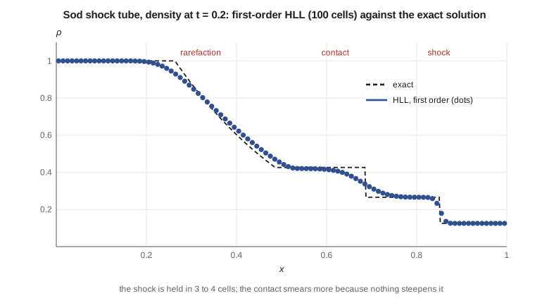
A shock tube is a long pipe with a diaphragm separating high-pressure gas from low-pressure gas. When the diaphragm bursts, a shock moves into the low-pressure gas, a rarefaction fan moves back into the high-pressure gas, and between them a contact surface separates gas that started on either side. The case defined by Gary Sod in 1978, with density and pressure of 1 on the left and 0.125 and 0.1 on the right, is a standard test because its exact solution can be computed by solving the Riemann problem. Arjun's code uses first-order HLL fluxes and compares the result with the exact solution.
# Sod shock tube: first-order finite-volume Euler solver with the HLL flux, checked against the exact Riemann solution.
import math
g = 1.4
def prim(U):
    r, m, E = U; u = m / r
    return r, u, (g - 1) * (E - 0.5 * r * u * u)
def flux(r, u, p):
    E = p / (g - 1) + 0.5 * r * u * u
    return (r * u, r * u * u + p, u * (E + p)), (r, r * u, E)
def hll(UL, UR):
    rl, ul, pl = prim(UL); rr, ur, pr = prim(UR)
    al, ar = math.sqrt(g * pl / rl), math.sqrt(g * pr / rr)
    sl, sr = min(ul - al, ur - ar), max(ul + al, ur + ar)    # Davis wave-speed estimates
    FL, _ = flux(rl, ul, pl); FR, _ = flux(rr, ur, pr)
    if sl >= 0: return FL
    if sr <= 0: return FR
    return tuple((sr * FL[k] - sl * FR[k] + sl * sr * (UR[k] - UL[k])) / (sr - sl) for k in range(3))
def exact_star(rl, ul, pl, rr, ur, pr):                     # Newton iteration for the star pressure (Toro)
    def fk(p, rk, pk):
        ak = math.sqrt(g * pk / rk)
        if p > pk:
            A, B = 2 / ((g + 1) * rk), (g - 1) / (g + 1) * pk
            return (p - pk) * math.sqrt(A / (p + B))
        return 2 * ak / (g - 1) * ((p / pk) ** ((g - 1) / (2 * g)) - 1)
    p = 0.5 * (pl + pr)
    for _ in range(50):
        F = fk(p, rl, pl) + fk(p, rr, pr) + ur - ul
        dp = 1e-7 * p
        dF = (fk(p + dp, rl, pl) + fk(p + dp, rr, pr) - fk(p - dp, rl, pl) - fk(p - dp, rr, pr)) / (2 * dp)
        p -= F / dF
    u = 0.5 * (ul + ur) + 0.5 * (fk(p, rr, pr) - fk(p, rl, pl))
    return p, u
L, R = (1.0, 0.0, 1.0), (0.125, 0.0, 0.1)                   # density, velocity, pressure
ps, us = exact_star(*L, *R)
rs_shock = R[0] * ((ps / R[2] + (g - 1) / (g + 1)) / ((g - 1) / (g + 1) * ps / R[2] + 1))
S = us * rs_shock / (rs_shock - R[0])                       # shock speed from mass conservation
print(f"Exact: p* = {ps:.5f}, u* = {us:.5f}, density behind shock {rs_shock:.5f}, shock speed {S:.5f}")
t_end, cfl = 0.2, 0.9
for n in (100, 400):
    dx = 1.0 / n; xs = [(i + 0.5) * dx for i in range(n)]
    U = [flux(*(L if x < 0.5 else R))[1] for x in xs]
    t = 0.0
    while t < t_end - 1e-12:
        smax = max(abs(prim(c)[1]) + math.sqrt(g * prim(c)[2] / prim(c)[0]) for c in U)
        dt = min(cfl * dx / smax, t_end - t)
        F = [hll(U[i], U[i + 1]) for i in range(n - 1)]
        U = [U[0]] + [tuple(U[i][k] - dt / dx * (F[i][k] - F[i - 1][k]) for k in range(3)) for i in range(1, n - 1)] + [U[-1]]
        t += dt
    P = [prim(c) for c in U]
    i_plateau = min(range(n), key=lambda i: abs(xs[i] - (0.5 + 0.5 * (us + S) * t_end)))
    x_shock = next(xs[i] for i in range(n - 1, 0, -1) if P[i][0] > 0.5 * (rs_shock + R[0]))
    print(f"N = {n:3d}: p in plateau {P[i_plateau][2]:.4f}, u {P[i_plateau][1]:.4f}, "
f"shock near x = {x_shock:.3f} (exact {0.5 + S * t_end:.3f})")Exact: p* = 0.30313, u* = 0.92745, density behind shock 0.26557, shock speed 1.75216 N = 100: p in plateau 0.3035, u 0.9286, shock near x = 0.845 (exact 0.850) N = 400: p in plateau 0.3032, u 0.9276, shock near x = 0.849 (exact 0.850)
The exact solution has a pressure of 0.30313 and a velocity of 0.92745 between the rarefaction and the shock, and the shock moves at 1.75216, reaching \(x = 0.850\) at \(t = 0.2\). With 100 cells, the HLL solver gets the plateau pressure within 0.1 per cent and places the shock within half a cell; with 400 cells, both converge further. The figure shows what the numbers do not: the shock is captured in three to four cells, sharp enough for most purposes, while the contact surface is spread over a dozen or more. A shock is self-steepening, because characteristics converge into it, and the numerical dissipation only fights a losing battle against that. A contact has no such mechanism, so dissipation smears it steadily. This is why HLLC or Roe fluxes are preferred whenever contacts or shear layers matter.
Boundary conditions
Boundary conditions for the Euler equations follow the characteristics. At a solid wall in an inviscid flow, the normal velocity is zero, and the flow slips tangentially; one condition is imposed and the wall pressure comes from the interior. At a far-field boundary, the number of conditions imposed from outside equals the number of incoming characteristics. For a subsonic inflow in three dimensions, four of the five characteristics enter and one, the \(u - c\) acoustic wave, leaves. Characteristic boundary conditions, often written in terms of Riemann invariants, impose the incoming values and extrapolate the outgoing ones, so that waves leave the domain without reflecting. A boundary that imposes all variables from the freestream reflects outgoing pressure waves back into the domain, which can stall convergence and corrupt lift.
| Boundary | Characteristics entering (3D) | Conditions imposed from outside |
|---|---|---|
| Supersonic inflow | 5 | All five variables |
| Subsonic inflow | 4 | For example total pressure, total temperature and two flow angles |
| Subsonic outflow | 1 | For example static pressure |
| Supersonic outflow | 0 | None; all variables extrapolated |
| Inviscid wall | 1 in effect | Zero normal velocity |
From the shock tube to the wing
The same algorithm, extended to three dimensions and to a body-fitted grid, solves the flow around the Swift 900 wing. Each cell face has an area and a normal vector, and the one-dimensional Riemann problem is solved in the direction normal to each face. Second-order accuracy comes from MUSCL reconstruction with limiters, and the steady state is reached by an implicit or multistage scheme with local time stepping. Kenji's three candidate sections are run at Mach 0.76 to 0.84 at the design lift coefficient. Section B keeps the upper-surface shock weakest, with a peak Mach number ahead of the shock of 1.18 at Mach 0.80 against 1.26 and 1.31 for the others, and shows the slowest drag rise.
The limits of the Euler model are clear to the high-speed group. Without a boundary layer, the computed shock sits too far aft, because the real boundary layer thickens through the shock and reduces the effective camber near the trailing edge. Lift at a given angle of attack is overpredicted, and the drag contains only wave drag and, in three dimensions, induced drag; there is no skin friction or form drag. A common remedy in the past was to couple an Euler solver with a boundary-layer code, a method called viscous-inviscid interaction, which remains useful in fast design tools. For the final Swift 900 wing, the group will use RANS, lesson 8 and 9, and keep Euler for screening and for loads at speeds where the boundary layer matters little.
Worked problem
Characteristic speeds at cruise
At the Swift 900 cruise point, \(u = 236\ \mathrm{m/s}\) and \(c = 295\ \mathrm{m/s}\). Find the three characteristic speeds and say which way each wave travels.
Show solution
- \(u - c = 236 - 295 = -59\ \mathrm{m/s}\): upstream.
- \(u = 236\ \mathrm{m/s}\): downstream, carried with the flow.
- \(u + c = 531\ \mathrm{m/s}\): downstream.
Answer: One upstream acoustic wave at 59 m/s and two downstream waves. The upstream wave is why a subsonic far field needs care.
Worked problem
HLL flux in a supersonic region
At a face in the supersonic pocket above the wing, \(u_L = 360\ \mathrm{m/s}\), \(c_L = 270\ \mathrm{m/s}\), \(u_R = 365\ \mathrm{m/s}\) and \(c_R = 268\ \mathrm{m/s}\). What does the HLL flux reduce to?
Show solution
- \(S_L = \min(360 - 270, 365 - 268) = 90\ \mathrm{m/s} > 0\).
- Both wave-speed estimates are positive, so all waves move right.
- The HLL formula gives \(\mathbf{F} = \mathbf{F}_L\).
Answer: The left, upwind flux. In fully supersonic flow, all upwind schemes reduce to the same one-sided flux.
Worked problem
Plateau error
The 100-cell HLL run gives a plateau pressure of 0.3035 against the exact 0.30313. What is the relative error, and what does it suggest?
Show solution
- Error: \((0.3035 - 0.30313)/0.30313 = 0.0012\), about 0.12 per cent.
- The plateau is a smooth constant state, so the error there is small even at first order.
- The larger errors sit at the waves, where first-order smearing acts.
Answer: About 0.1 per cent. Integrated quantities depend on the whole field, so a grid study is still needed.
Common mistakes
MistakeEuler solutions give total drag.
InsteadThey give wave and induced drag only; skin friction and form drag need a viscous model.
MistakeFixing all freestream values at the far field is safest.
InsteadOver-specifying reflects outgoing waves; use characteristic conditions.
MistakeA sharp shock in the solution means the contact and shear layers are sharp too.
InsteadShocks self-steepen; contacts and shear layers do not and smear unless the flux resolves them.
MistakeIn subsonic flow, one upwind direction works for all variables.
InsteadWaves travel both upstream and downstream; each wave family must be upwinded separately.
Summary and key terms
- The Euler equations are a hyperbolic system with wave speeds \(u - c\), \(u\) and \(u + c\), so numerical methods must treat each wave family by the sign of its speed.
- Flux-vector splitting, Roe, HLL and HLLC fluxes, and central schemes with artificial dissipation such as JST, are the main approaches.
- The Sod shock tube tests a solver against an exact solution and shows that shocks are captured sharply while contacts smear.
- Boundary conditions must match the incoming characteristics.
- Euler solutions screen transonic designs quickly but omit viscous effects that move shocks and add drag.
- Flux Jacobian
- The matrix of derivatives of the flux with respect to the conserved variables; its eigenvalues are the wave speeds.
- Flux-vector splitting
- Splitting the flux into parts carried by positive and negative waves.
- HLL flux
- An approximate Riemann flux assuming a single state between the fastest waves.
- JST scheme
- A central scheme with blended second- and fourth-difference artificial dissipation.
- Shock tube
- A test problem in which a diaphragm separates gases at different pressures.
- Contact surface
- A surface separating gases of different density at equal pressure and velocity.
- Characteristic boundary condition
- A condition that imposes incoming wave values and extrapolates outgoing ones.
Practice problems
Work each problem on paper first, then reveal the answer to check.
How many conditions are imposed at a subsonic outflow in three dimensions?
Show answer
One, usually static pressure.
Why does the contact surface smear more than the shock?
Show answer
A shock is self-steepening; a contact is not, so numerical dissipation spreads it steadily.
What does HLL lack that HLLC restores?
Show answer
The contact wave in the middle of the Riemann fan.
Why does an Euler solution put the transonic shock too far aft?
Show answer
It omits the boundary layer, which thickens at the shock and reduces effective camber.
What is the exact Sod shock position at \(t = 0.2\)?
Show answer
\(x = 0.5 + 1.75216 \times 0.2 = 0.850\).
Lesson quiz · 5 questions
Score 60% or more to complete this lesson.
Create a free account to save your progress, take quizzes and earn a certificate.