
AERO-440 · Lesson 1 of 12 · 28 min
Why CFD
Every aerodynamics course so far has leaned on two kinds of evidence: theory that can be worked by hand, such as thin-airfoil theory and lifting-line theory, and measurements from the National Research Council 9 m wind tunnel in Ottawa. Both remain essential, but neither answers every question that a modern aircraft program asks. Borealis Aerospace in Winnipeg has three such programs on the table at once. The Petrel 19 is the 19-seat hybrid commuter whose concept design was set in the aircraft design course. The Tern Block 2 is the updated wing for the existing Tern utility aircraft, tested at one-third scale in the tunnel. The Swift 900 is the light business jet study that must cruise at Mach 0.80. Each program now needs answers that hand methods cannot give and that tunnel time alone cannot afford.
Tomasz Wierzbicki, head of aerodynamics, has been given the budget to set up a computational fluid dynamics group. Arjun Mehta, now an engineer in training after his final co-op term, joins the group full time. Dr. Kenji Watanabe brings the transonic questions from the high-speed group, Marcus Webb needs pressure loads for the structure, Hélène Lavoie needs an aerodynamic database for the flight simulator, and Rachel Oduya, the certification manager, wants to know how much of this Transport Canada will accept as evidence. This course follows the group through its first year, from the equations themselves to the day a CFD result changes a design decision.
What CFD is
Computational fluid dynamics, or CFD, is the numerical solution of the equations that govern fluid flow. Those equations, conservation of mass, momentum and energy, were written down in the nineteenth century. For anything but the simplest geometries they cannot be solved exactly. CFD replaces the continuous flow field with values stored at a finite number of points or in a finite number of small cells, replaces derivatives and integrals with algebraic approximations, and solves the resulting very large system of equations on a computer. The answer is never exact: it carries errors from the geometry, from the grid, from the numerical method, from incomplete convergence and from the physical model. Much of this course is about understanding those errors well enough to trust, or distrust, a result.
The word computational is easy to underrate. The equations of fluid motion are nonlinear, they couple pressure, velocity, density and temperature, and their solutions contain features ranging from a shock wave a fraction of a millimetre thick to a wake several wingspans long. A useful three-dimensional simulation of a wing at cruise uses tens of millions of cells and solves for five or more unknowns in each. That is why CFD grew with computing power, and why it is still shaped by what can be computed overnight on the hardware a company can afford.
A short history
Numerical methods for flow are older than electronic computers. Lewis Fry Richardson attempted a numerical weather forecast by hand during the First World War, and Richard Courant, Kurt Friedrichs and Hans Lewy published their analysis of stability for difference equations in 1928. The condition that bears their initials, the CFL condition, appears in lesson 5. In the 1960s, panel methods such as the one developed by John Hess and A. M. O. Smith at Douglas let engineers compute the inviscid pressure on complete aircraft surfaces. In 1970, Earll Murman and Julian Cole showed how to compute transonic flows with embedded shocks by switching the difference scheme where the flow became supersonic, and through the 1970s and 1980s Antony Jameson's codes made Euler and then Navier-Stokes solutions of wings practical. By the 1990s, Reynolds-averaged Navier-Stokes solvers with one- and two-equation turbulence models were in routine industrial use, and they remain the workhorse today.
The other half of the history is cost. A calculation that occupied a national laboratory's computer for a weekend in the early 1980s now runs on a workstation in minutes. The cost of a given simulation has fallen by many orders of magnitude, while the cost of tunnel and flight testing has not. This shift did not make testing obsolete, but it changed the role of each tool.
What CFD offers and what it does not
CFD offers things a tunnel cannot. It gives the full flow field, not just the quantities a balance or a pressure tap can measure. It has no wall interference, no model support, and no limit on Reynolds number other than cost. It can run full-scale flight conditions, including the high Reynolds numbers that small tunnels cannot reach. Geometry changes cost hours rather than weeks of model shop time. It can isolate one effect, such as removing the nacelle to see what the wing does alone, in a way that no physical test can.
CFD also has limits that matter. Its answers depend on models of turbulence and transition that are calibrated for attached flows and become unreliable as separation grows. The grid controls the accuracy, and an inexperienced user can produce smooth, colourful pictures from a grid that is far too coarse. Iterative solvers can stall or converge to the wrong answer. A simulation that has not been verified and validated is a sophisticated guess. The group's first rule, written by Tomasz on the whiteboard, is that a CFD result is a claim that must be supported, not a measurement that speaks for itself.
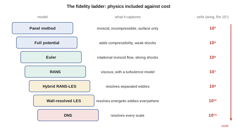
The hierarchy of models
Engineers choose among several levels of physical model. Panel methods solve Laplace's equation for an inviscid, incompressible, irrotational flow and need only the surface to be divided into panels; they run in seconds and are still used for early design and for loads. Full-potential methods add compressibility and can capture weak shocks. The Euler equations are the full inviscid conservation laws; they capture strong shocks, vorticity and rotational flow, but not boundary layers. The Reynolds-averaged Navier-Stokes equations, or RANS, add viscosity and model the effect of turbulence on the mean flow; most industrial CFD on aircraft is RANS. Hybrid methods such as detached-eddy simulation use RANS near walls and resolve large eddies in separated regions. Large-eddy simulation, or LES, resolves the energetic eddies everywhere and models only the small ones. Direct numerical simulation, or DNS, resolves every scale of turbulence and needs no turbulence model at all.
The cost rises steeply along this ladder. A widely used estimate for DNS is that the number of grid points scales with the Reynolds number to the power nine-quarters. For wall-resolved LES of a boundary layer, Choi and Moin estimated a power of about thirteen-sevenths. The code below applies these estimates to the Tern Block 2 wing at cruise and also classifies the governing equations, which is the first question to ask of any equation one intends to solve numerically.
# Classify second-order PDEs a*u_xx + b*u_xy + c*u_yy = f by the discriminant b^2 - 4ac,
# then apply it to the small-disturbance potential equation (1 - M^2) phi_xx + phi_yy = 0.
# Finally, compare rough grid-point counts for DNS, wall-resolved LES and RANS on the Tern Block 2 wing.
def classify(a, b, c):
    d = b * b - 4 * a * c
    if abs(d) < 1e-12:
        return "parabolic"
    return "hyperbolic" if d > 0 else "elliptic"

print("Model equations")
print("  Laplace      u_xx + u_yy = 0        :", classify(1, 0, 1))
print("  Wave         u_tt - c^2 u_xx = 0    :", classify(-4.0, 0, 1))
print("  Heat         u_t = nu u_xx (t as y) :", classify(1, 0, 0))
print()
print("Small-disturbance potential equation, (1 - M^2) phi_xx + phi_yy = 0")
for M in (0.32, 0.80, 1.00, 1.40, 2.00):
    kind = classify(1 - M * M, 0, 1)
    print(f"  M = {M:4.2f}: coefficient of phi_xx = {1 - M*M:+.3f} -> {kind}")
print()
# Grid estimates (order of magnitude): DNS ~ Re^(9/4) for the whole flow (Kolmogorov scaling),
# wall-resolved LES ~ Re^(13/7) (Choi and Moin 2012), RANS ~ 1e7 for a clean wing-body case.
Re = 9.8e6        # Tern Block 2 cruise, based on the 1.73 m mean aerodynamic chord
dns = Re ** (9 / 4)
les = Re ** (13 / 7)
rans = 1.0e7
print(f"Tern Block 2 cruise Reynolds number: {Re:.2e}")
print(f"  DNS grid points (Re^9/4)          : {dns:.1e}")
print(f"  wall-resolved LES points (Re^13/7): {les:.1e}")
print(f"  typical RANS wing-body mesh       : {rans:.1e}")
print(f" DNS / RANS ratio : {dns / rans:.1e}")Model equations Laplace u_xx + u_yy = 0 : elliptic Wave u_tt - c^2 u_xx = 0 : hyperbolic Heat u_t = nu u_xx (t as y) : parabolic Small-disturbance potential equation, (1 - M^2) phi_xx + phi_yy = 0 M = 0.32: coefficient of phi_xx = +0.898 -> elliptic M = 0.80: coefficient of phi_xx = +0.360 -> elliptic M = 1.00: coefficient of phi_xx = +0.000 -> parabolic M = 1.40: coefficient of phi_xx = -0.960 -> hyperbolic M = 2.00: coefficient of phi_xx = -3.000 -> hyperbolic Tern Block 2 cruise Reynolds number: 9.80e+06 DNS grid points (Re^9/4) : 5.4e+15 wall-resolved LES points (Re^13/7): 9.6e+12 typical RANS wing-body mesh : 1.0e+07 DNS / RANS ratio : 5.4e+08
The output makes two points. First, the type of equation changes with Mach number: the small-disturbance potential equation is elliptic below Mach 1 and hyperbolic above it. Elliptic problems spread information in all directions, so every point affects every other; hyperbolic problems carry information along characteristic directions at finite speed. A numerical method must respect this, which is the whole reason Murman and Cole's switched scheme worked for transonic flow. Second, DNS of the Tern Block 2 wing would need something like \(10^{15}\) grid points, roughly eight orders of magnitude more than a RANS mesh. That gap is why turbulence models, imperfect as they are, remain central to aircraft CFD.
Where CFD fits beside testing
Modern aircraft programs use CFD, wind tunnels and flight test as complementary tools. CFD is cheap per configuration and is used to explore many options and to understand the flow. The tunnel is used to check a smaller number of configurations, to measure quantities that CFD predicts poorly, such as maximum lift and buffet onset, and to calibrate the CFD. Flight test confirms the final aircraft. As CFD has matured, the number of tunnel hours per program has fallen, but no transport aircraft has yet been certified on CFD alone.
| Question | Best first tool | Why |
|---|---|---|
| Pressure distribution on the Tern Block 2 wing at cruise | RANS CFD | Attached flow; full field; flight Reynolds number |
| Maximum lift with flaps deployed | Tunnel, then flight test | Separation and transition dominate; CFD scatter is large |
| Swift 900 drag rise from Mach 0.70 to 0.84 | RANS CFD, checked in a transonic tunnel | Shock position is sensitive; many Mach numbers needed |
| Petrel 19 nacelle and wing interference | RANS CFD | Isolating components is easy; tunnel can confirm the total |
| Stall behaviour and spin resistance | Flight test, with tunnel support | Unsteady, separated, dynamic; certification requires flight |
| First look at forty planform options | Panel or vortex-lattice method | Seconds per case; trends matter more than absolute values |
The CFD workflow
Every CFD calculation passes through the same stages. The geometry is taken from the computer-aided design model and cleaned up: small gaps are closed, tiny features that do not affect the aerodynamics are removed, and the surfaces are made watertight. A grid, or mesh, is built around the geometry. The flow solver then iterates toward a solution of the discretized equations. The results are post-processed into forces, moments, pressure distributions and pictures of the flow. Finally, the results are judged: is the solution converged, is the grid fine enough, and does it agree with trusted data where such data exist? Each stage introduces errors of its own.
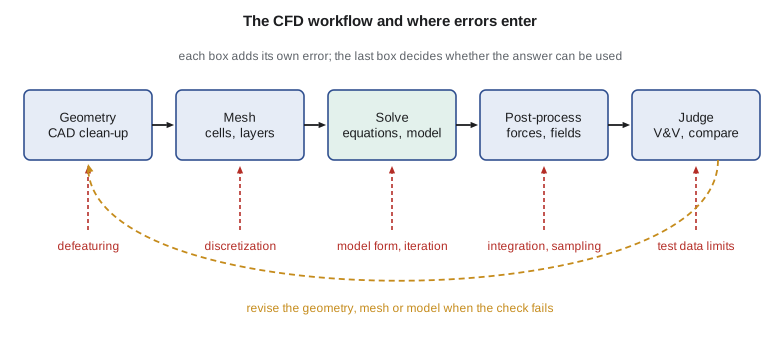
In practice the mesh and the judgement take most of the engineer's time. For a new configuration, building a good mesh can take days while the solver runs overnight. Industry experience, gathered in the AIAA Drag Prediction Workshops and High Lift Prediction Workshops, shows that the spread between different groups' answers for the same geometry often comes more from meshing and user choices than from the solvers themselves. The group therefore writes down its practices: how first-cell heights are chosen, how many prism layers are used, what residual reduction counts as converged, and which turbulence model is the default.
Codes and tools
The group surveys the codes available. Open-source solvers include SU2, which began at Stanford University and is widely used for aerodynamic shape design, and OpenFOAM, a general finite-volume toolbox used across many industries. NASA has developed and supports codes such as FUN3D, an unstructured-grid solver, and CFL3D, a structured-grid solver with a long validation record; access to these codes is controlled, and their use depends on the user's eligibility. Commercial packages such as Ansys Fluent and Siemens STAR-CCM+ offer integrated meshing, solving and post-processing with vendor support. Each has strengths; none removes the need to understand what it is doing. The group decides to run one commercial package for production work and SU2 for research and design studies, and to write small codes of its own, like those in this course, to understand the algorithms.
Worked problem
Choosing a model level
Arjun is asked for the lift-curve slope of three candidate Tern Block 2 planforms by the end of the day, with no flaps and at cruise conditions. Which model level should he use?
Show solution
- The flow is attached and the question is about trends in a linear quantity.
- A vortex-lattice or panel method gives lift-curve slope well for attached flow and runs in seconds.
- RANS would add viscous effects that change the slope only slightly, at hours per case.
- The tunnel data from AERO-300 can check the baseline planform.
Answer: A vortex-lattice or panel method, checked against the baseline tunnel slope. RANS is not needed for this question.
Worked problem
Estimating the DNS gap
The code gives about \(5.4 \times 10^{15}\) grid points for DNS of the Tern Block 2 wing at a Reynolds number of \(9.8 \times 10^{6}\). If a RANS run on \(10^{7}\) cells takes 4 hours on the group's computer, and cost scales with cell count, how long would DNS take?
Show solution
- The ratio of cells is \(5.4 \times 10^{15} / 10^{7} = 5.4 \times 10^{8}\).
- DNS also needs far smaller time steps and long averaging, so the true ratio is larger still.
- Even on cell count alone: \(4 \times 5.4 \times 10^{8} = 2.2 \times 10^{9}\) hours, about 250 000 years.
Answer: About 250 000 years on cell count alone. DNS of a flight-Reynolds-number wing is not a design tool.
Worked problem
Equation type at the Swift 900 cruise
Kenji says that at Mach 0.80 the Swift 900 wing has a pocket of supersonic flow above the upper surface. What type is the small-disturbance potential equation inside and outside that pocket, and what does that mean for the numerical method?
Show solution
- Outside the pocket, the local Mach number is below 1, so \(1 - M^2 > 0\) and the equation is elliptic.
- Inside the pocket, \(M > 1\), so \(1 - M^2 < 0\) and the equation is hyperbolic.
- The method must use upwind differences in the hyperbolic region so information travels downstream only.
Answer: Elliptic outside, hyperbolic inside. The scheme must change its character with the local Mach number, as Murman and Cole's did.
Common mistakes
MistakeA CFD result is accurate because the picture looks smooth and plausible.
InsteadSmooth contours can come from a coarse grid or an unconverged solution. Accuracy must be shown by grid studies and by comparison with trusted data.
MistakeCFD replaces wind tunnel and flight testing.
InsteadCFD reduces the number of tests and guides them, but separated flows, maximum lift and certification still depend on tests.
MistakeHigher-fidelity models are always better.
InsteadA higher model level costs far more. The right level is the cheapest one that captures the physics that matter for the question.
MistakeThe solver is the main source of disagreement between groups.
InsteadWorkshop experience shows that meshing practice and user choices often cause more scatter than the solvers themselves.
Summary and key terms
- CFD solves the conservation laws of fluid flow numerically on a grid, and its answers carry errors from geometry, grid, method, convergence and physical model.
- Panel methods, full-potential methods, Euler, RANS, hybrid RANS-LES, LES and DNS form a ladder of increasing physics and cost.
- RANS is the industrial workhorse because DNS at flight Reynolds numbers would need about \(10^{15}\) points.
- The type of the governing equations, elliptic, parabolic or hyperbolic, decides how information travels and how a method must be built.
- CFD, tunnels and flight test are complementary tools, and every CFD result must be judged before it is used.
- CFD
- Computational fluid dynamics: the numerical solution of the equations of fluid flow.
- RANS
- Reynolds-averaged Navier-Stokes: equations for the mean flow, with turbulence represented by a model.
- LES
- Large-eddy simulation: large eddies resolved, small eddies modelled.
- DNS
- Direct numerical simulation: all scales of turbulence resolved, no turbulence model.
- Elliptic equation
- An equation in which every point influences every other; typical of subsonic steady flow.
- Hyperbolic equation
- An equation with characteristic directions along which information travels at finite speed; typical of supersonic flow and unsteady inviscid flow.
- Panel method
- A boundary-element method that solves for inviscid flow using singularities on the body surface.
Practice problems
Work each problem on paper first, then reveal the answer to check.
Classify \(u_{xx} + 4u_{xy} + u_{yy} = 0\).
Show answer
\(b^2 - 4ac = 16 - 4 = 12 > 0\): hyperbolic.
Classify the small-disturbance potential equation at Mach 0.5 and Mach 1.5.
Show answer
\(1 - M^2 = 0.75\) gives elliptic at Mach 0.5; \(1 - M^2 = -1.25\) gives hyperbolic at Mach 1.5.
Using the nine-quarters scaling, by what factor do DNS grid points grow when the Reynolds number rises tenfold?
Show answer
\(10^{9/4} \approx 178\).
Name two quantities that CFD predicts less reliably than lift-curve slope.
Show answer
Maximum lift and buffet onset, both of which depend on separation.
Why does a CFD group write down meshing and convergence practices?
Show answer
Because user choices cause much of the scatter between results, and written practices make results repeatable and reviewable.
Lesson quiz · 5 questions
Score 60% or more to complete this lesson.
Create a free account to save your progress, take quizzes and earn a certificate.