
AERO-440 · Lesson 6 of 12 · 24 min
Grid generation
Six weeks into the group's life, Arjun has learned what every CFD engineer learns: the solver runs overnight, but the grid takes the week. The first full configuration the group tackles is the Tern Block 2 wing on its fuselage at cruise, the same shape that was tested at one-third scale in the National Research Council 9 m wind tunnel in Ottawa, so the CFD can later be compared with tunnel data. Tomasz sets the target: a grid that resolves the boundary layer down to the wall, captures the wingtip vortex for two spans downstream, and can be refined systematically for the grid study in lesson 10. This lesson covers how grids are built and what makes one good.
Why the grid matters
The grid decides what the solver can see. Features smaller than a few cells, a thin boundary layer, a shock, a vortex core, cannot be resolved, and errors in one region spread to others. The truncation error analysis of lesson 2 assumed uniform spacing; on a real grid, sudden changes in cell size or shape add errors of their own, and highly skewed cells degrade both accuracy and convergence. A grid that is fine where gradients are large and coarse where the flow is uniform puts the cells where they matter. Industry workshop results consistently show that grid quality and resolution account for a large share of the variation between groups computing the same aircraft.
Structured grids
A structured grid has a regular index structure: every interior point has neighbours at \(i \pm 1\), \(j \pm 1\) and \(k \pm 1\), like a deformed block of graph paper. The connectivity is implicit, so memory use is low and line-based implicit solvers and multigrid are natural. Structured grids give excellent quality in boundary layers, because grid lines can follow the wall and stretch away from it smoothly. Around a two-dimensional airfoil, the classic topologies are the O-grid, which wraps around the body and closes on itself; the C-grid, which wraps around the nose and continues downstream along the wake, so that wake resolution is natural; and the H-grid, made of lines running roughly streamwise and normal to the flow.
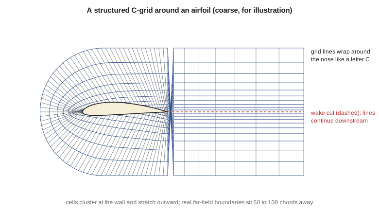
Structured grids are generated by mapping. In algebraic methods, interior points are interpolated from boundary points; transfinite interpolation blends the four boundary curves of a two-dimensional block, or the six faces of a three-dimensional one, into a smooth interior. Clustering toward walls is controlled by stretching functions such as geometric progressions or hyperbolic tangents. In elliptic methods, the grid coordinates are found by solving Poisson equations, whose smoothing property gives very smooth grids, with source terms that control spacing and orthogonality at the walls. Hyperbolic methods march outward from the body surface, layer by layer, and give near-orthogonal grids quickly, though they offer little control over the outer boundary.
For a complete aircraft, a single structured block is impossible. The domain is divided into many blocks, each structured, joined at their faces: a multiblock grid. A wing-body-nacelle configuration can need hundreds of blocks, and building the block topology is skilled, slow work. Overset, or chimera, grids relax this: separate grids around each component overlap, and the solver interpolates between them in the overlap regions. Overset grids are widely used for moving bodies, such as store separation and rotors, and for complex configurations where blocking would be impractical.
Unstructured grids
An unstructured grid stores its connectivity explicitly, so any cell shape and arrangement is possible. Tetrahedra fill any volume and can be generated automatically, by Delaunay triangulation, which connects points so that no point lies inside the circumsphere of any tetrahedron, or by advancing front methods, which grow cells layer by layer from the surface into the volume. Automatic generation is the great advantage: a complex geometry that would take weeks to block can be meshed in hours. The cost is more memory per cell, more irregular data access and, for tetrahedra in boundary layers, poor accuracy, because thin tetrahedra have bad angles.
The standard compromise is the hybrid grid. Layers of prisms, triangular in the surface and stacked normal to the wall, or of hexahedra on quadrilateral surface meshes, are extruded from the surface to resolve the boundary layer with high-aspect-ratio cells aligned with the flow. Tetrahedra, or general polyhedra, fill the rest of the domain, with pyramids where quadrilateral faces meet triangular ones. Commercial packages and open-source mesh generators such as those used with SU2 and OpenFOAM build such grids routinely. Polyhedral grids, made by merging tetrahedra into larger cells with many faces, have fewer cells for the same accuracy and are standard in some commercial solvers. Cartesian cut-cell methods take a different route: a simple Cartesian grid fills the domain, and cells intersected by the body are cut to fit it. They are almost fully automatic and are used for rapid inviscid analysis, but the boundary layer needs special treatment.
Resolving the boundary layer: first cell height and y+
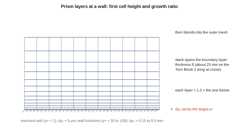
The boundary layer sets the hardest requirement. Its velocity profile rises from zero at the wall to the edge velocity over a thickness of millimetres to centimetres, and the steepest part lies within a few micrometres of the wall. Turbulence models that integrate to the wall, lesson 9, require the centre of the first cell to sit at a nondimensional wall distance \(y^{+}\) of about 1. Wall functions, which bridge the inner layer with an analytical profile, instead want \(y^{+}\) between about 30 and 100.
The friction velocity \(u_\tau\) depends on the wall shear stress, which is not known before the solution. It is estimated from a flat-plate skin-friction correlation at the relevant Reynolds number. The code below does this for the Tern Block 2 wing at its cruise condition, Mach 0.32 at 3000 m, and for the Swift 900 at Mach 0.80 and 12 500 m, using White's correlation \(C_f = 0.026/Re_x^{1/7}\). It then counts the prism layers needed to span the boundary layer thickness at several growth ratios, and checks a hyperbolic tangent stretching function.
# First-cell height for a target y+ and a geometric prism-layer stack, using flat-plate turbulent correlations.
import math
def isa(h):                                   # troposphere and lower stratosphere, h in m
    T = 288.15 - 0.0065 * min(h, 11000.0)
    p = 101325 * (T / 288.15) ** 5.2559 if h <= 11000 else 22632.1 * math.exp(-(h - 11000) / 6341.6)
    rho = p / (287.05 * T)
    mu = 1.458e-6 * T ** 1.5 / (T + 110.4)    # Sutherland's law
    return T, rho, mu, math.sqrt(1.4 * 287.05 * T)
cases = (("Tern Block 2 cruise", 3000.0, 0.32, 1.73), ("Swift 900 cruise", 12500.0, 0.80, 2.40))
for name, h, M, c in cases:
    T, rho, mu, a = isa(h)
    V = M * a; Re = rho * V * c / mu
    Cf = 0.026 / Re ** (1 / 7)                # White's turbulent skin friction at x = c
    tau = 0.5 * rho * V * V * Cf
    ut = math.sqrt(tau / rho); nu = mu / rho
    delta = 0.37 * c / Re ** 0.2              # turbulent boundary-layer thickness at x = c
    print(f"{name}: V = {V:.1f} m/s, Re_c = {Re:.2e}, Cf = {Cf:.5f}, u_tau = {ut:.3f} m/s")
    for yp in (1.0, 30.0):
        y1 = yp * nu / ut
        print(f"  y+ = {yp:4.0f}: first cell height {y1 * 1e6:8.2f} micrometres")
    y1 = nu / ut
    for r in (1.15, 1.20, 1.25):              # growth ratio of the prism layers
        n = math.ceil(math.log(1 + delta * (r - 1) / y1) / math.log(r))
        print(f"  growth {r:.2f}: {n:2d} layers to span delta = {delta * 1000:.1f} mm")
    print()
# Tanh clustering of 41 points across [0, 1] toward both ends (a common algebraic stretching)
beta, N = 2.5, 41
s = [0.5 * (1 + math.tanh(beta * (2 * k / (N - 1) - 1)) / math.tanh(beta)) for k in range(N)]
d = [s[k + 1] - s[k] for k in range(N - 1)]
print(f"tanh stretching, beta = {beta}: end spacing {d[0]:.5f}, mid spacing {d[N // 2]:.5f}, "
f"largest neighbour ratio {max(max(d[k+1]/d[k], d[k]/d[k+1]) for k in range(N - 2)):.3f}")Tern Block 2 cruise: V = 105.1 m/s, Re_c = 9.76e+06, Cf = 0.00261, u_tau = 3.798 m/s y+ = 1: first cell height 4.91 micrometres y+ = 30: first cell height 147.18 micrometres growth 1.15: 48 layers to span delta = 25.6 mm growth 1.20: 39 layers to span delta = 25.6 mm growth 1.25: 33 layers to span delta = 25.6 mm Swift 900 cruise: V = 236.1 m/s, Re_c = 1.14e+07, Cf = 0.00255, u_tau = 8.429 m/s y+ = 1: first cell height 5.87 micrometres y+ = 30: first cell height 176.13 micrometres growth 1.15: 49 layers to span delta = 34.4 mm growth 1.20: 39 layers to span delta = 34.4 mm growth 1.25: 33 layers to span delta = 34.4 mm tanh stretching, beta = 2.5: end spacing 0.00191, mid spacing 0.06302, largest neighbour ratio 1.278
For \(y^{+} = 1\), the first cell on the Tern Block 2 wing must be about 5 micrometres thick, roughly a twentieth of a human hair, on a wing with a 1.73 m mean chord. The Swift 900 needs about 6 micrometres. With a growth ratio of 1.2, about 39 layers span the 25 to 35 mm boundary layer at the trailing edge. These numbers explain why boundary-layer grids have cells with aspect ratios of 1000 or more: the cells are perhaps 5 mm long in the flow direction and a few micrometres thick. They also show why the first-cell height is set by a calculation, not by eye. The tanh function clusters points smoothly, with a largest neighbour ratio of about 1.28 for the chosen parameter, inside the usual guideline.
Grid quality
Several measures of quality are checked before a grid is used. Skewness measures how far a cell departs from an ideal shape; highly skewed cells reduce accuracy and slow convergence, and solvers often fail on cells with skewness near 1. Orthogonality measures the angle between the line joining two cell centres and the face between them; non-orthogonality introduces errors in gradient and diffusion terms. Growth ratio, the ratio of neighbouring cell sizes, should usually stay below about 1.2 to 1.3 in regions of high gradients. Aspect ratio may be very high in a boundary layer, where it follows the flow, but should be moderate elsewhere. Negative volumes, cells turned inside out by a bad mapping, make a grid unusable.
| Region of the Tern Block 2 grid | Practice adopted by the group |
|---|---|
| Wall-normal first cell | \(y^+ \approx 1\): 5 micrometres at cruise |
| Prism layer growth | 1.2, about 40 layers, then smooth blend into the volume mesh |
| Chordwise spacing at leading and trailing edges | About 0.1 per cent of local chord |
| Trailing edge | Blunt base resolved with at least 8 cells across |
| Wingtip and vortex wake | Refinement region two spans long, at least 20 cells across the core |
| Far-field boundary | 100 mean chords from the aircraft |
| Cell count, medium grid | About 12 million cells for the half model |
The far-field distance matters more than beginners expect. A lifting wing induces a velocity field that decays slowly with distance, and a far-field boundary only a few chords away constrains the circulation and changes the lift and induced drag. The group places the boundary 100 mean chords away, where the coarse cells cost little, and confirms that moving it farther changes drag by less than a tenth of a count. Vortex-based far-field corrections can reduce the distance required.
Adaptation
A grid built before the solution is known can only guess where the gradients will be. Solution-adaptive refinement splits cells where an error indicator, such as a large density gradient or a large estimated truncation error, is high, and may coarsen cells elsewhere. Adjoint-based adaptation goes further: it refines where local errors most affect a chosen output, such as drag, and can reach a given accuracy in that output with far fewer cells. Kenji's group uses gradient-based adaptation to sharpen the Swift 900 upper-surface shock, which a fixed grid smears over several cells.
Worked problem
First cell height for a new condition
Arjun needs a grid for the Tern Block 2 at its approach condition: 55 m/s at sea level, where \(\nu = 1.46 \times 10^{-5}\ \mathrm{m^2/s}\) and the chord is 1.73 m. Find the first-cell height for \(y^+ = 1\).
Show solution
- \(Re = 55 \times 1.73 / 1.46 \times 10^{-5} = 6.52 \times 10^{6}\).
- \(C_f = 0.026 / (6.52 \times 10^{6})^{1/7} = 0.026/9.41 = 0.00276\).
- \(u_\tau = V\sqrt{C_f/2} = 55 \times 0.0372 = 2.04\ \mathrm{m/s}\).
- \(y = 1 \times 1.46 \times 10^{-5}/2.04 = 7.2 \times 10^{-6}\ \mathrm{m}\).
Answer: About 7 micrometres. Lower speed means a thicker first cell for the same \(y^+\).
Worked problem
Layers to span the boundary layer
With a first cell of 5 micrometres and a growth ratio of 1.2, how thick is the stack after 30 layers?
Show solution
- Geometric series: \(\Delta y_1 (r^{n} - 1)/(r - 1)\).
- \(5 \times 10^{-6} \times (1.2^{30} - 1)/0.2 = 5 \times 10^{-6} \times 1182\).
- Stack height: 5.9 mm.
Answer: 5.9 mm, well short of the 25 mm boundary layer; about 39 layers are needed, as the code found.
Worked problem
Choosing a topology
Marcus asks whether the Petrel 19 nacelle-pylon-wing junction should be meshed with structured multiblock or hybrid unstructured grids. The geometry will change several times during the design.
Show solution
- Multiblock topology for a junction is slow to build and must be rebuilt for each major change.
- Hybrid unstructured grids can be regenerated automatically from the new geometry.
- Prism layers keep boundary-layer quality near the walls.
Answer: Hybrid unstructured, with prism layers at the walls, because the geometry is still changing and automation matters more than the last bit of grid quality.
Common mistakes
MistakeUse the same first-cell height for every flight condition.
InsteadThe required height depends on the Reynolds number and changes with speed and altitude; recompute it for each condition.
MistakeA finer grid everywhere is the safest choice.
InsteadUniform refinement wastes cells where the flow is smooth; refine where gradients and outputs demand it.
MistakePlace the far-field boundary a few chords away to save cells.
InsteadLifting flows need distant boundaries, typically 50 to 100 chords, or a vortex correction.
MistakeHigh aspect ratio cells are always bad.
InsteadThey are appropriate in boundary layers if aligned with the flow; skewness and abrupt growth are the real problems.
Summary and key terms
- The grid decides what the solver can resolve and is the largest single source of variation between CFD results.
- Structured grids give efficient, high-quality boundary layers but need multiblock topology for complex shapes; unstructured and hybrid grids mesh complex shapes automatically, with prism layers for the boundary layer.
- The first-cell height comes from the target \(y^+\) and an estimate of skin friction.
- Quality checks cover skewness, orthogonality, growth ratio and far-field distance, and adaptation puts cells where errors are largest.
- Structured grid
- A grid with implicit i, j, k connectivity.
- Unstructured grid
- A grid with explicitly stored connectivity, allowing any cell arrangement.
- Hybrid grid
- Prism or hexahedral layers at walls with tetrahedral or polyhedral cells elsewhere.
- Overset grid
- Overlapping component grids that exchange data by interpolation.
- y+
- Wall distance scaled by the friction velocity and kinematic viscosity.
- Growth ratio
- The ratio of the sizes of neighbouring cells.
- Skewness
- A measure of how far a cell departs from its ideal shape.
Practice problems
Work each problem on paper first, then reveal the answer to check.
What first-cell height gives \(y^+ = 30\) on the Tern Block 2 at cruise?
Show answer
About 0.15 mm, from the code.
Which structured topology resolves the wake of an airfoil most naturally?
Show answer
The C-grid.
How many layers with growth 1.25 span 25.6 mm from a 4.9 micrometre first cell?
Show answer
About 33, from the code.
Why are thin tetrahedra poor in boundary layers?
Show answer
They have bad angles and misaligned faces, which harm gradient accuracy; prisms aligned with the wall are far better.
What does adjoint-based adaptation refine?
Show answer
The cells whose local errors most affect a chosen output, such as drag.
Lesson quiz · 5 questions
Score 60% or more to complete this lesson.
Create a free account to save your progress, take quizzes and earn a certificate.