Finite difference methods

With truncation error understood, Arjun builds his first working solvers. The test problem is the linear advection equation on a periodic domain: whatever leaves the right boundary re-enters at the left, so after one period the exact solution is the initial profile again. Any change in shape is purely numerical error. Tomasz chooses two profiles. A smooth Gaussian bump tests accuracy, and a square pulse with sharp edges stands in for the shock waves and contact surfaces that the Swift 900 solver will have to capture. The results set the pattern for everything that follows: the trade between accuracy on smooth flow and clean behaviour at discontinuities.

Explicit schemes for advection

An explicit scheme computes each new value directly from known values at the old time level. Writing the Courant number as \(\nu = a\,\Delta t/\Delta x\), the distance the wave moves in one step measured in cells, the main explicit schemes for \(u_t + a u_x = 0\) with \(a > 0\) are these.

FTCS, forward in time and central in space, looks natural but is unstable for advection, as lesson 2 noted. The upwind scheme takes the spatial difference from the side the wave comes from. It is first order and stable for \(0 \le \nu \le 1\). Lax-Friedrichs replaces \(u_i^n\) in FTCS by the average of its neighbours, which makes it stable for \(|\nu| \le 1\) but adds heavy smoothing. Lax-Wendroff is derived by expanding \(u^{n+1}\) in a Taylor series in time to second order and using the equation itself to replace the time derivatives with space derivatives: \(u_{tt} = a^{2}u_{xx}\). The result is the FTCS scheme plus a diffusion-like correction, second order in both space and time, and stable for \(|\nu| \le 1\).

Upwinding is a central idea in CFD. For a hyperbolic equation, information travels along characteristics. A scheme that takes its information from the direction the characteristic comes from respects the physics. One that takes information symmetrically, or from downstream, does not, and must be stabilized by other means. When \(a < 0\), the upwind scheme uses \(u_{i+1}\) instead of \(u_{i-1}\). For systems such as the Euler equations, with waves moving both ways at once, upwinding requires splitting the flux by wave direction, which is the subject of lessons 4 and 7.

A numerical experiment

# Linear advection u_t + a u_x = 0 on a periodic domain [0, 1], a = 1, one full trip around (t = 1).
# Compare first-order upwind, Lax-Friedrichs and second-order Lax-Wendroff on a smooth Gaussian and a square pulse.
import math
def run(scheme, u0, nu, steps):
    u = u0[:]; n = len(u)
    for _ in range(steps):
        v = u[:]
        for i in range(n):
            um, up = u[i - 1], u[(i + 1) % n]
            if scheme == "upwind":
                v[i] = u[i] - nu * (u[i] - um)
            elif scheme == "Lax-Friedrichs":
                v[i] = 0.5 * (up + um) - 0.5 * nu * (up - um)
            else:  # Lax-Wendroff
                v[i] = u[i] - 0.5 * nu * (up - um) + 0.5 * nu * nu * (up - 2 * u[i] + um)
        u = v
    return u
def initial(kind, n):
    xs = [(i + 0.5) / n for i in range(n)]
    if kind == "gauss":
        return [math.exp(-((x - 0.5) / 0.08) ** 2) for x in xs]
    return [1.0 if 0.3 <= x <= 0.7 else 0.0 for x in xs]
nu = 0.5                      # Courant number a*dt/dx
for kind in ("gauss", "square"):
    print(f"{kind} profile, Courant number {nu}, after one period")
    print("  scheme            N   L1 error    max     min")
    for scheme in ("upwind", "Lax-Friedrichs", "Lax-Wendroff"):
        for n in (50, 200):
            u0 = initial(kind, n)
            u = run(scheme, u0, nu, int(round(n / nu)))
            err = sum(abs(a - b) for a, b in zip(u, u0)) / n
            print(f"  {scheme:15s} {n:3d}   {err:.4f}   {max(u):.3f}  {min(u):+.3f}")
    print()
# Observed order of accuracy from the Gaussian L1 errors
for scheme in ("upwind", "Lax-Wendroff"):
    e = []
    for n in (100, 200, 400):
        u0 = initial("gauss", n); u = run(scheme, u0, nu, int(round(n / nu)))
        e.append(sum(abs(a - b) for a, b in zip(u, u0)) / n)
    print(f"{scheme:13s} observed order (smooth data): {math.log(e[0]/e[1], 2):.2f}, {math.log(e[1]/e[2], 2):.2f}")

gauss profile, Courant number 0.5, after one period
  scheme            N   L1 error    max     min
  upwind           50   0.0939   0.490  +0.000
  upwind          200   0.0394   0.749  +0.000
  Lax-Friedrichs   50   0.1441   0.310  +0.014
  Lax-Friedrichs  200   0.0805   0.547  +0.000
  Lax-Wendroff     50   0.0490   0.887  -0.123
  Lax-Wendroff    200   0.0037   0.997  -0.000

square profile, Courant number 0.5, after one period
  scheme            N   L1 error    max     min
  upwind           50   0.1592   0.954  +0.003
  upwind          200   0.0797   1.000  +0.000
  Lax-Friedrichs   50   0.2730   0.751  +0.082
  Lax-Friedrichs  200   0.1381   0.979  +0.001
  Lax-Wendroff     50   0.1167   1.204  -0.204
  Lax-Wendroff    200   0.0523   1.232  -0.232

upwind        observed order (smooth data): 0.69, 0.80
Lax-Wendroff  observed order (smooth data): 1.96, 2.00

The results show the character of each scheme. On the Gaussian with 50 cells, the upwind scheme reduces the peak from 1 to 0.49; it has smeared the profile badly. Lax-Friedrichs is worse, at 0.31. Lax-Wendroff keeps the peak at 0.89 but overshoots below zero, to −0.12. With 200 cells, Lax-Wendroff's error has fallen by a factor of about 13 and the peak is almost exact, while upwind is still at 0.75. The observed order on the smooth profile, about 2 for Lax-Wendroff and below 1 for upwind on these coarse grids, confirms the theory. Upwind's order rises toward 1 as the grid is refined.

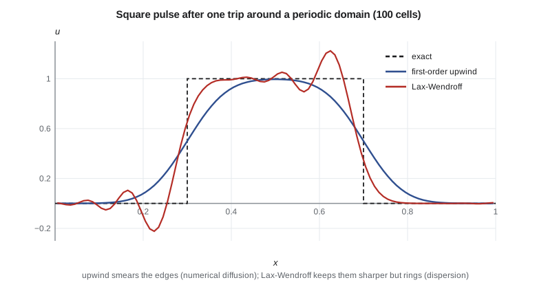
On the square pulse, the picture changes. Upwind and Lax-Friedrichs keep the solution between 0 and 1: no new maxima or minima appear. Lax-Wendroff overshoots to 1.23 and undershoots to −0.23, and refining the grid does not remove the overshoot; the oscillations simply become narrower. For a density or pressure, an undershoot below zero is not just ugly, it is unphysical and can crash a solver.

The modified equation

Why do the schemes behave so differently? The modified equation answers that. Substitute Taylor series into the difference scheme and find the differential equation it actually solves to higher order. For the upwind scheme, the result is

The upwind scheme solves the advection equation plus a diffusion term with coefficient \(a\Delta x(1-\nu)/2\). This numerical diffusion, sometimes called artificial viscosity, is why the Gaussian spreads and decays. It is also why the scheme is stable: diffusion damps oscillations. The coefficient is positive only for \(\nu \le 1\), and it vanishes at \(\nu = 1\), where the upwind scheme simply shifts the profile one cell per step and is exact. For Lax-Wendroff, the leading error term is a third derivative, \(-\tfrac{a\Delta x^{2}}{6}(1 - \nu^{2})u_{xxx}\). A third-derivative term is dispersive rather than diffusive: it makes waves of different wavelength travel at different speeds. A sharp edge contains all wavelengths, so they separate and appear as a train of ripples behind the jump.

The modified equation also explains a practical problem. For the upwind scheme, the numerical viscosity is proportional to \(\Delta x\). On the Tern Block 2 wing at cruise, the physical kinematic viscosity is about \(1.9 \times 10^{-5}\ \mathrm{m^2/s}\). With a velocity of 105 m/s and a cell size of 5 mm, the upwind numerical viscosity at a small Courant number is about \(0.26\ \mathrm{m^2/s}\), more than ten thousand times larger. A first-order upwind solution of a boundary layer on such a grid would compute the flow of a very viscous fluid. This is why production codes use second-order schemes, and why first-order solutions are used only to start a calculation.

Godunov's theorem

The square-pulse results are not an accident of the particular schemes. In 1959 Sergei Godunov proved that a linear scheme that never creates new extrema, called monotone or monotonicity-preserving, can be at most first-order accurate. A designer cannot have both second-order accuracy and freedom from oscillations with a linear scheme. The way around the theorem is to make the scheme nonlinear: second order where the solution is smooth and first order near discontinuities, with the switch controlled by the solution itself. These high-resolution schemes, built with flux limiters or slope limiters, are the foundation of modern shock-capturing and are introduced in lesson 4.

Implicit methods for diffusion

The diffusion equation \(u_t = \nu u_{xx}\) can be solved explicitly with forward time and central space differences, but stability requires \(r = \nu\Delta t/\Delta x^{2} \le 1/2\). The time step must shrink with the square of the cell size. In a boundary-layer grid, where wall cells may be a few micrometres thick, this restriction would make explicit time stepping hopelessly slow. Implicit methods evaluate the spatial derivative at the new time level, or at a mix of old and new. The backward Euler scheme is

Each new value now depends on its unknown neighbours, so the scheme gives a system of equations to solve at every step. In one dimension the system is tridiagonal: each row has nonzero entries only on the diagonal and its two neighbours. Such systems are solved directly in a number of operations proportional to the number of unknowns by the Thomas algorithm, a streamlined form of Gaussian elimination. Backward Euler is unconditionally stable but only first order in time. The Crank-Nicolson scheme averages the old and new spatial differences, giving second order in time and unconditional stability, at the cost of some oscillation when very large time steps meet sharp initial data.

In two and three dimensions the implicit systems are no longer tridiagonal. Approximate factorization, such as the alternating direction implicit method, splits a multidimensional step into a sequence of one-dimensional tridiagonal solves. The Beam-Warming scheme of the 1970s applied this idea to the compressible Navier-Stokes equations and made implicit structured-grid solvers practical; codes in the CFL3D family descend from that line of work.

Higher-order and compact schemes

Wider stencils give higher-order accuracy. The five-point central difference from lesson 2 is fourth order. Compact schemes achieve high order on narrow stencils by relating the derivatives at neighbouring points as well as the function values; they need a tridiagonal solve but give excellent resolution of short waves. They are used in DNS and LES on simple domains, where errors must be far smaller than in RANS. For complex aircraft geometries, most production solvers remain second order, because the accuracy is limited more by the grid and the turbulence model than by the scheme order.