
AERO-440 · Lesson 12 of 12 · 25 min
Using CFD in design
By the end of its first year, the group's work has shifted from answering questions about fixed shapes to helping choose the shapes themselves. The Swift 900 wing planform is still open: the high-speed group has fixed the section and the sweep, but the taper ratio and the tip washout, the twist that lowers the tip's angle of attack relative to the root, are to be chosen. Lower drag pulls one way, the wing-root bending moment that Marcus must carry in the structure pulls another, and every evaluation is an overnight RANS run. This final lesson shows how CFD is used inside a design process, from parametric geometry to surrogate models and adjoint optimization, and how its results are carried into decisions and certification.
CFD in the design cycle
In the conceptual phase, decisions are made quickly on many options with low-fidelity tools: handbook methods, vortex-lattice and panel methods. In preliminary design, the configuration is settled and RANS becomes the main aerodynamic tool, with tunnel tests to confirm. In detailed design, CFD supplies loads for the structure, the aerodynamic database for flight simulation and handling, and analyses of specific problems such as ice shapes, antenna placement and cabin air intakes. The right tool changes with the phase, and a common mistake is to use high-fidelity CFD too early, on a configuration whose layout has not been fixed, or too late, after the tunnel model has already been built.
Hélène's needs illustrate the scale of a database task. The flight simulator for the Swift 900 needs forces and moments across Mach number, angle of attack, sideslip and control deflections: tens of thousands of conditions. RANS cannot fill such a table alone. The group runs RANS at a few hundred well-chosen points, uses a panel method and the tunnel for the rest, and fits a smooth model that blends them, with RANS anchoring the high-speed and high-angle corners where simpler methods fail.
Parametric geometry and automation
To use CFD in a design loop, the geometry must be described by a small number of design variables, such as taper ratio, twist at a few span stations, thickness and camber parameters, or the coefficients of shape functions that deform the surface smoothly. The free-form deformation and class-shape transformation methods are common choices. Each change in the variables must flow automatically through geometry generation, meshing, solving and post-processing without manual intervention. Automation is often the hardest part. Mesh generation that needs a human for each new shape breaks the loop, so the group uses either automatic hybrid meshing or mesh deformation, in which the existing grid is moved smoothly to follow the new surface, keeping its topology and the prism-layer structure intact.
Design of experiments and surrogate models
When each evaluation costs hours, the number of evaluations is the budget. A surrogate model, also called a response surface or metamodel, is a cheap approximation fitted to a modest number of expensive evaluations. The evaluations are placed by a design of experiments: a full factorial grid for two or three variables, or a Latin hypercube or similar space-filling design for more. Common surrogates are polynomial response surfaces, radial basis functions and kriging, also known as Gaussian process regression, which also estimates its own uncertainty and so can indicate where the next evaluation would be most informative.
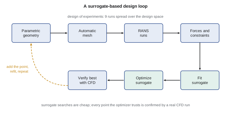
The procedure, often called surrogate-based optimization, runs in a loop. Fit the surrogate to the evaluations made so far. Search the surrogate, which is cheap, for the best design that meets the constraints. Evaluate that design with the real CFD. Add the result to the data and refit. Stop when the surrogate's prediction at its optimum agrees with the CFD there and the design stops moving. The code below demonstrates the loop on the Swift 900 planform problem with a quadratic response surface. A simple analytical function stands in for the RANS drag so that the example runs in a second; in the real study each call was a RANS run of about four hours. The constraint is that the wing-root bending moment must not exceed that of the baseline design.
# A surrogate-based design loop. The "CFD" function below stands in for a RANS run that returns the cruise drag
# (counts) of a wing with tip washout w (deg) and taper ratio t; each call is treated as costing hours.
# A quadratic response surface is fitted to a 3 x 3 design of experiments, its minimum is found, the minimum is
# checked with a new "CFD" run, the point is added, and the surface is refitted.
import math
calls = 0
def cfd(w, t):
    global calls; calls += 1
    return 246.0 + 0.9 * (w - 3.2)**2 + 150.0 * (t - 0.50)**2 + 3.0 * (w - 3.2) * (t - 0.50) + 0.6 * math.sin(2.2 * w) + 400.0 * (t - 0.50)**3
def root_moment(w, t):          # wing-root bending moment relative to the baseline; must stay <= 1.00
    return 1.0 - 0.030 * (w - 1.0) + 0.55 * (t - 0.35)
def basis(w, t): return [1.0, w, t, w * w, t * t, w * t]
def fit(pts):                   # least squares via the normal equations
    n = 6; A = [[0.0]*n for _ in range(n)]; b = [0.0]*n
    for w, t, f in pts:
        phi = basis(w, t)
        for i in range(n):
            b[i] += phi[i] * f
            for j in range(n): A[i][j] += phi[i] * phi[j]
    for c in range(n):
        r = max(range(c, n), key=lambda q: abs(A[q][c])); A[c], A[r] = A[r], A[c]; b[c], b[r] = b[r], b[c]
        for q in range(c + 1, n):
            k = A[q][c] / A[c][c]; b[q] -= k * b[c]
            for j in range(c, n): A[q][j] -= k * A[c][j]
    x = [0.0]*n
    for c in range(n - 1, -1, -1): x[c] = (b[c] - sum(A[c][j]*x[j] for j in range(c + 1, n))) / A[c][c]
    return lambda w, t: sum(ci * pi for ci, pi in zip(x, basis(w, t)))
def best(model):                # dense search of the surrogate inside bounds, with the bending constraint
    cand = [(0.5 + 4.0 * i / 120, 0.30 + 0.30 * j / 120) for i in range(121) for j in range(121)]
    ok = [c for c in cand if root_moment(*c) <= 1.0]
    return min(ok, key=lambda c: model(*c))
pts = [(w, t, cfd(w, t)) for w in (0.5, 2.5, 4.5) for t in (0.30, 0.45, 0.60)]
print("Design of experiments: 9 CFD runs, baseline (w 1.0, t 0.35) drag", f"{cfd(1.0, 0.35):.2f} counts")
for it in range(1, 5):
    model = fit(pts)
    w, t = best(model)
    f = cfd(w, t)
    print(f"  iteration {it}: surrogate optimum w = {w:.3f} deg, t = {t:.4f}; predicted {model(w, t):.2f}, "
          f"CFD {f:.2f} counts, root moment {root_moment(w, t):.3f}")
    pts.append((w, t, f))
print(f"Total CFD runs: {calls} (the baseline evaluation included)")
grid = min(((0.5 + 4.0*i/60, 0.30 + 0.30*j/60) for i in range(61) for j in range(61)
            if root_moment(0.5 + 4.0*i/60, 0.30 + 0.30*j/60) <= 1.0), key=lambda c: cfd(*c))
print(f"Brute-force check on a 61 x 61 grid ({61*61} runs): w = {grid[0]:.3f}, t = {grid[1]:.3f}, drag {cfd(*grid):.2f}")Design of experiments: 9 CFD runs, baseline (w 1.0, t 0.35) drag 253.86 counts iteration 1: surrogate optimum w = 3.267 deg, t = 0.4650; predicted 245.80, CFD 246.63 counts, root moment 0.995 iteration 2: surrogate optimum w = 3.267 deg, t = 0.4675; predicted 246.07, CFD 246.61 counts, root moment 0.997 iteration 3: surrogate optimum w = 3.267 deg, t = 0.4675; predicted 246.21, CFD 246.61 counts, root moment 0.997 iteration 4: surrogate optimum w = 3.300 deg, t = 0.4675; predicted 246.29, CFD 246.64 counts, root moment 0.996 Total CFD runs: 14 (the baseline evaluation included) Brute-force check on a 61 x 61 grid (3721 runs): w = 2.833, t = 0.450, drag 246.47
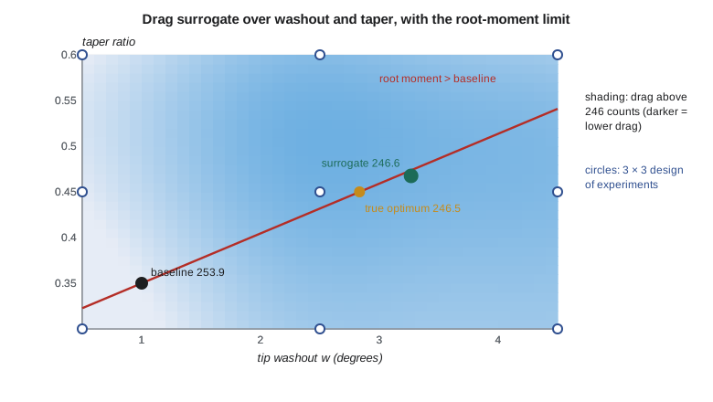
The baseline wing, with 1 degree of washout and a taper ratio of 0.35, has a drag of 253.9 counts. After the nine-run design of experiments, the first surrogate optimum lies at 3.27 degrees of washout and a taper ratio of 0.465, with a predicted drag of 245.8 counts. The confirming CFD run gives 246.6 counts: the surrogate had underpredicted the drag by 0.8 counts. With each added point, the surrogate's prediction at its optimum approaches the CFD value, and the design settles. In 14 evaluations the loop has saved 7.2 counts against the baseline while keeping the root moment just inside the limit. A brute-force search with 3721 evaluations, impossible with real CFD, finds a true constrained optimum of 246.47 counts at a somewhat different point. The best design the loop evaluated, at 246.61 counts, is within 0.14 counts of it, a gap smaller than the numerical uncertainty of the RANS drag from lesson 10.
The gap between the surrogate and the brute-force optimum illustrates two points. A single global quadratic cannot follow a function with local wiggles, so the surrogate is biased; kriging or a trust-region method that refits locally around the current best design would close the gap. And the drag surface near the optimum is flat: points differing by half a degree of washout differ by a fraction of a count. Flat optima are common in aerodynamic design, and they are good news, because they give room to satisfy other requirements, such as stall behaviour or manufacturing, at little cost in drag.
Adjoint methods
Surrogates work well for a handful of variables, but the number of evaluations needed grows quickly with the number of variables. Detailed wing shape design may use hundreds of variables. Gradient-based optimization needs the derivative of the objective, such as drag, with respect to every variable. Finite differences would cost one extra CFD run per variable. The adjoint method computes all these derivatives for the cost of one additional solution, of the adjoint equations, roughly the cost of the flow solution itself, regardless of the number of design variables. Antony Jameson introduced adjoint methods to aerodynamic shape design in the late 1980s, and they are now standard in SU2 and several other codes. The adjoint solution has a physical meaning too: it shows how sensitive the objective is to changes at every point in the flow, and it is the basis of the adjoint-based grid adaptation mentioned in lesson 6.
Adjoint-based optimization is powerful but needs care. The optimizer will exploit any weakness in the model, for example by shaping the wing to delay separation in a way the turbulence model rewards but real flow would not. Constraints on thickness, volume, pitching moment and off-design performance must be imposed, or the optimizer will produce a wing that is excellent at one point and poor elsewhere. Multipoint optimization, which minimizes a weighted sum of drag at several Mach numbers and lift coefficients, gives more robust designs. Every optimized shape is checked at off-design conditions and, ultimately, in the tunnel.
Uncertainty and decisions
Design decisions are only as good as the confidence in the numbers behind them. A drag difference of 2 counts between two designs means little if the numerical and model uncertainty of each is larger, unless the uncertainty is common to both and cancels in the increment. The group reports each design comparison as an increment with its own uncertainty, estimated from grid studies of both designs and from the spread between two turbulence models. Kenji's rule is that a CFD-driven change goes into the design only if the predicted gain exceeds twice the uncertainty of the increment, or if it is confirmed in the tunnel.
| Use of CFD | Phase | Typical confidence | Check |
|---|---|---|---|
| Planform and twist trades | Preliminary | High for increments | Grid study, two turbulence models |
| Transonic drag rise | Preliminary and detailed | Medium | Transonic tunnel test |
| Structural loads at attached conditions | Detailed | High | Pressure-tapped tunnel model, flight strain gauges |
| Maximum lift and stall | Detailed | Low to medium | Tunnel and flight test |
| Simulator database | Detailed | Varies with region | Tunnel data and flight test matching |
| Certification evidence | Certification | Supporting, not standalone | Validated against tests on similar configurations |
CFD and certification
Rachel's plan with Transport Canada uses CFD in three ways. It supports the selection of critical conditions for flight and structural tests, so that the tests cover the worst cases. It interpolates and extrapolates between tested conditions, for example loads at weights and centre-of-gravity positions not flown, where validation at the tested points supports the analysis between them. And it supports small design changes, where a validated CFD increment from a tested baseline can reduce the need to repeat tests, subject to the authority's agreement. In each case, the credibility argument of lesson 10 is what makes CFD acceptable: a documented, verified and validated process applied within its validated range. The group's practices document, which began as Tomasz's whiteboard rule a year earlier, has become part of the company's compliance procedures.
Looking ahead
The field continues to move. Wall-modelled LES and hybrid methods are approaching routine use for high-lift and buffet. Graphics-processor computing has cut run times for many solvers by large factors. Machine learning is being explored for turbulence-model corrections, for surrogates trained on large databases of CFD runs and for faster mesh generation, with the same need for verification and validation as any other model. The NASA CFD Vision 2030 study, published in 2014, set out goals for this progress, including reliable prediction of separated flows and automated, error-controlled simulation. None of this changes the core of what the group has learned: understand the equations and the algorithm, build grids with care, know the limits of the physical model, measure the numerical error, compare with trusted data, and state the uncertainty with every answer.
Worked problem
Cost of a finite-difference gradient
A wing has 120 shape variables. A RANS run takes 4 hours and an adjoint solution takes 5 hours. Compare the cost of one gradient by forward finite differences and by the adjoint method.
Show solution
- Finite differences: one baseline run plus 120 perturbed runs: \(121 \times 4 = 484\) hours.
- Adjoint: one flow run plus one adjoint run: \(4 + 5 = 9\) hours.
- Ratio: about 54.
Answer: About 484 hours against 9 hours. The adjoint cost does not grow with the number of variables.
Worked problem
Is the design change justified?
Two Swift 900 wing designs differ by 2.4 counts in predicted drag. The uncertainty of the increment, from grid studies and the spread between two turbulence models, is 0.9 counts. Does Kenji's rule allow the change?
Show solution
- Twice the uncertainty is \(2 \times 0.9 = 1.8\) counts.
- The predicted gain of 2.4 counts exceeds 1.8 counts.
Answer: Yes. The gain exceeds twice its uncertainty, so the change can go into the design, with tunnel confirmation planned.
Worked problem
Surrogate error
In the first loop iteration, the surrogate predicted 245.80 counts and the CFD gave 246.63 counts. In the last, the prediction was 246.29 and the CFD 246.64. How has the surrogate's error changed, and what does it suggest?
Show solution
- First error: \(246.63 - 245.80 = 0.83\) counts.
- Last error: \(246.64 - 246.29 = 0.35\) counts.
- The error has fallen as points cluster near the optimum, but a bias remains because a global quadratic cannot follow local wiggles.
Answer: The error fell from 0.83 to 0.35 counts. A local or kriging surrogate would reduce it further.
Common mistakes
MistakeUse the highest-fidelity CFD from the start of a design.
InsteadHigh fidelity is wasted on layouts that will change; match the tool to the phase.
MistakeA surrogate's optimum is the true optimum.
InsteadSurrogates are approximations; every candidate must be confirmed with real CFD, and biases checked.
MistakeAn optimizer's result can go straight to the tunnel.
InsteadOptimizers exploit model weaknesses; check off-design performance, constraints and physical plausibility first.
MistakeCFD alone can show compliance with certification requirements.
InsteadCFD supports tests and is accepted within its validated range, with the authority's agreement; it does not replace demonstration tests.
Summary and key terms
- CFD's role changes through the design cycle, from low-fidelity trades in conceptual design to RANS in preliminary design and loads and databases in detailed design.
- Parametric geometry and automated meshing allow CFD to run inside design loops.
- Surrogate-based optimization fits cheap models to a design of experiments and confirms each candidate with CFD; the adjoint method gives gradients for many variables at the cost of one extra solution.
- Design changes are accepted when predicted gains exceed their uncertainty, and CFD supports certification within its validated range.
- Design variable
- A parameter that defines the geometry in an optimization.
- Design of experiments
- A plan for placing expensive evaluations across the design space.
- Surrogate model
- A cheap approximation fitted to expensive evaluations.
- Kriging
- A surrogate based on Gaussian process regression that also estimates its uncertainty.
- Adjoint method
- A way to compute the gradient of one output with respect to many variables at the cost of one extra solution.
- Multipoint optimization
- Optimization over several flight conditions at once for robust designs.
- Mesh deformation
- Moving an existing grid to follow a changed surface without regenerating it.
Practice problems
Work each problem on paper first, then reveal the answer to check.
How many runs does a full factorial design need for three variables at three levels?
Show answer
\(3^{3} = 27\).
Why does kriging help choose the next evaluation?
Show answer
It estimates its own uncertainty, so points can be placed where the prediction is least certain or most promising.
What is the main cost advantage of the adjoint method?
Show answer
The gradient costs about one extra solution, independent of the number of design variables.
Why is a flat optimum useful in design?
Show answer
It allows other requirements to be met with little drag penalty.
Name one way CFD supports certification.
Show answer
Selecting critical conditions for tests, interpolating between tested conditions, or supporting small design changes from a validated baseline.
Lesson quiz · 5 questions
Score 60% or more to complete this lesson.
Create a free account to save your progress, take quizzes and earn a certificate.