
AERO-440 · Lesson 2 of 12 · 27 min
Model equations and discretization
Before the group runs a single wing, Tomasz insists that everyone understand what a solver actually does to the equations. The full Navier-Stokes equations are too complicated to study directly, so CFD is taught, and its methods are designed, using model equations: simple equations that each keep one essential feature of the real ones. Arjun spends his first two weeks with four of them, a notebook and a laptop. This lesson sets out the conservation laws, the model equations, and the basic idea of discretization, and it measures the truncation error that every approximation carries.
The conservation laws
Fluid flow obeys three conservation laws. Mass is neither created nor destroyed. The rate of change of momentum of a fluid parcel equals the sum of the forces on it, pressure and viscous stresses. Energy changes by the work done and the heat added. Written for a fixed control volume \(V\) with surface \(S\), each law has the same form: the rate of change of the conserved quantity inside the volume plus the net flux of that quantity out through the surface equals any source inside.
Here \(\mathbf{U}\) is the vector of conserved variables: density, the three components of momentum per unit volume, and total energy per unit volume. \(\mathbf{F}\) is the flux, which contains both a convective part, carried by the flow, and a diffusive part from viscosity and heat conduction. If the solution is smooth, the divergence theorem turns the integral form into a differential form, \(\partial \mathbf{U}/\partial t + \nabla\cdot\mathbf{F} = \mathbf{Q}\). The distinction matters: the integral form remains valid across a shock wave, where derivatives do not exist, while the differential form does not. Finite-volume methods, lesson 4, are built on the integral form for exactly this reason.
A form in which the time derivative acts on the conserved variables and the spatial derivatives act on fluxes is called conservation form. Mathematically equivalent forms written in terms of velocity, pressure and temperature, sometimes called primitive or non-conservative forms, give the same smooth solutions but different, wrong shock speeds when discretized. The Lax-Wendroff theorem states that if a conservative scheme converges as the grid is refined, it converges to a weak solution of the conservation law, which includes the correct shock jumps. That theorem is the reason almost every compressible-flow code is written in conservation form.
Four model equations
The first model equation is linear advection, \(u_t + a u_x = 0\). It describes a profile carried at constant speed \(a\) without changing shape, and its exact solution is \(u(x,t) = u_0(x - at)\). It is the simplest hyperbolic equation and the model for how waves and disturbances are convected through a flow. The lines \(x - at = \text{constant}\) are its characteristics: the solution is constant along them.
The second is the diffusion equation, \(u_t = \nu u_{xx}\). It is parabolic and models the smoothing effect of viscosity and heat conduction. An initial spike spreads out and decays; information travels at infinite speed but with exponentially small amplitude far away. The third is the inviscid Burgers equation, \(u_t + (u^2/2)_x = 0\), which is advection with a speed equal to the solution itself. Faster parts of the profile overtake slower parts, so a smooth profile can steepen into a shock in finite time. Burgers' equation is the standard model for the nonlinearity of the Euler equations. Adding diffusion gives the viscous Burgers equation, \(u_t + u u_x = \nu u_{xx}\), which models the balance between steepening and viscosity inside a shock or a boundary layer. The fourth is Laplace's equation, \(u_{xx} + u_{yy} = 0\), the elliptic model for steady subsonic potential flow and the equation that panel methods solve.
| Model equation | Type | Feature of the full equations it models |
|---|---|---|
| \(u_t + a u_x = 0\) | Hyperbolic | Convection of disturbances at finite speed |
| \(u_t = \nu u_{xx}\) | Parabolic | Viscous and thermal diffusion |
| \(u_t + (u^2/2)_x = 0\) | Hyperbolic, nonlinear | Steepening into shocks; shock speed |
| \(u_t + u u_x = \nu u_{xx}\) | Mixed | Shock structure; boundary-layer balance |
| \(u_{xx} + u_{yy} = 0\) | Elliptic | Steady subsonic potential flow |
Discretization
To solve any of these on a computer, the continuous domain is replaced by a grid. In one dimension, the points are \(x_i = i\,\Delta x\), and time advances in steps \(t^n = n\,\Delta t\). The unknown \(u(x_i, t^n)\) is approximated by a number \(u_i^n\). The differential equation is then replaced by an algebraic relation among nearby values, called a difference equation, and the set of points it involves is called its stencil.
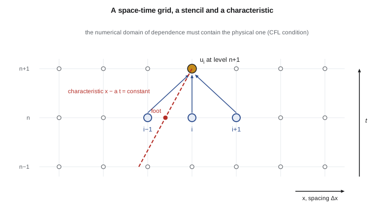
There are three main families of discretization. Finite-difference methods approximate derivatives at grid points using Taylor series; they are simple and efficient on smooth structured grids, and lesson 3 covers them. Finite-volume methods divide the domain into cells and balance fluxes through the cell faces; they are naturally conservative and work on any cell shape, which is why nearly all aerodynamic production codes use them. Finite-element methods represent the solution as a combination of basis functions over each element and require the residual to be orthogonal to a set of test functions; they dominate structural analysis and are increasingly used in high-order flow solvers. All three lead to large systems of algebraic equations.
Taylor series and truncation error
The building block of finite differences is the Taylor series. Expanding \(u\) about \(x_i\):
Rearranging gives the forward difference \((u_{i+1} - u_i)/\Delta x = u_x + (\Delta x/2)\,u_{xx} + \cdots\). The extra terms on the right are the truncation error: the difference between the difference formula and the derivative it replaces. Its leading term is proportional to \(\Delta x\), so the forward difference is first-order accurate. Subtracting the expansion for \(u_{i-1}\) from that for \(u_{i+1}\) cancels the even terms and gives the central difference, whose leading error is \((\Delta x^{2}/6)\,u_{xxx}\): second order. Adding the two expansions gives the standard approximation to the second derivative, also second order, with leading error \((\Delta x^{2}/12)\,u_{xxxx}\).
Order of accuracy describes how the error falls as the grid is refined. Halving \(\Delta x\) halves the error of a first-order formula and quarters the error of a second-order one. This gives a practical test that will reappear in verification, lesson 10: compute with several spacings, and see whether the error falls at the rate the theory predicts. If it does not, there is a bug or the solution is not smooth enough. The code below does this for \(u = \sin x\), where the exact derivatives are known.
# Truncation error of finite-difference approximations to du/dx and d2u/dx2 for u = sin(x) at x = 1.
# The observed order p is found from successive grid halvings: p = log(e_h / e_h/2) / log 2.
import math
u = math.sin
x0 = 1.0
exact1 = math.cos(x0)      # du/dx
exact2 = -math.sin(x0)     # d2u/dx2
schemes = {
    "forward  (u[i+1]-u[i])/h        ": lambda h: (u(x0 + h) - u(x0)) / h,
    "backward (u[i]-u[i-1])/h        ": lambda h: (u(x0) - u(x0 - h)) / h,
    "central  (u[i+1]-u[i-1])/2h     ": lambda h: (u(x0 + h) - u(x0 - h)) / (2 * h),
    "4th-order central (5 points)    ": lambda h: (-u(x0 + 2*h) + 8*u(x0 + h) - 8*u(x0 - h) + u(x0 - 2*h)) / (12 * h),
}
hs = [0.2 / 2**k for k in range(5)]
print("First derivative of sin(x) at x = 1, exact =", f"{exact1:.10f}")
for name, f in schemes.items():
    errs = [abs(f(h) - exact1) for h in hs]
    orders = [math.log(errs[k] / errs[k + 1], 2) for k in range(len(hs) - 1)]
    print(f"  {name} error at h=0.0125: {errs[-1]:.2e}  observed order: " + " ".join(f"{p:.2f}" for p in orders))
print()
print("Second derivative (u[i+1] - 2u[i] + u[i-1])/h^2, exact =", f"{exact2:.10f}")
prev = None
for h in hs:
    d2 = (u(x0 + h) - 2 * u(x0) + u(x0 - h)) / h**2
    e = abs(d2 - exact2)
    lead = abs(h * h / 12 * math.sin(x0))   # leading truncation term h^2/12 * u''''
    tag = "" if prev is None else f"  ratio {prev / e:.2f}"
    print(f"  h = {h:.4f}: error {e:.3e}, predicted h^2/12 u'''' = {lead:.3e}{tag}")
    prev = e
print()
# Too small a step: round-off grows as eps/h and swamps the truncation error.
print("Round-off limit for the central first derivative")
for h in (1e-2, 1e-4, 1e-6, 1e-8, 1e-10):
    e = abs((u(x0 + h) - u(x0 - h)) / (2 * h) - exact1)
print(f" h = {h:.0e}: error {e:.1e}")First derivative of sin(x) at x = 1, exact = 0.5403023059 forward (u[i+1]-u[i])/h error at h=0.0125: 5.27e-03 observed order: 1.03 1.01 1.01 1.00 backward (u[i]-u[i-1])/h error at h=0.0125: 5.25e-03 observed order: 0.96 0.98 0.99 1.00 central (u[i+1]-u[i-1])/2h error at h=0.0125: 1.41e-05 observed order: 2.00 2.00 2.00 2.00 4th-order central (5 points) error at h=0.0125: 4.40e-10 observed order: 3.99 4.00 4.00 4.00 Second derivative (u[i+1] - 2u[i] + u[i-1])/h^2, exact = -0.8414709848 h = 0.2000: error 2.801e-03, predicted h^2/12 u'''' = 2.805e-03 h = 0.1000: error 7.010e-04, predicted h^2/12 u'''' = 7.012e-04 ratio 4.00 h = 0.0500: error 1.753e-04, predicted h^2/12 u'''' = 1.753e-04 ratio 4.00 h = 0.0250: error 4.383e-05, predicted h^2/12 u'''' = 4.383e-05 ratio 4.00 h = 0.0125: error 1.096e-05, predicted h^2/12 u'''' = 1.096e-05 ratio 4.00 Round-off limit for the central first derivative h = 1e-02: error 9.0e-06 h = 1e-04: error 9.0e-10 h = 1e-06: error 2.8e-11 h = 1e-08: error 2.6e-09 h = 1e-10: error 5.8e-08
The observed orders match the theory: about 1 for the one-sided differences, 2 for the central difference and 4 for the five-point formula. For the second derivative, the error ratio is exactly 4 per halving and the error itself matches the predicted leading term \(\Delta x^{2}u_{xxxx}/12\) to three figures. The last block shows a limit that every numerical engineer meets sooner or later. As \(h\) shrinks below about \(10^{-6}\), the error grows again, because subtracting two nearly equal numbers loses significant digits. Round-off error grows like \(\varepsilon/h\), where \(\varepsilon\) is about \(10^{-16}\) in double precision, while truncation error falls like \(h^2\). Real CFD grids never approach this limit in space, but the same effect appears when derivatives are estimated by finite differences of a solver's output, as in some design sensitivity calculations.
Consistency, stability and convergence
Three properties decide whether a scheme is useful. A scheme is consistent if its truncation error goes to zero as \(\Delta x\) and \(\Delta t\) go to zero; it then approximates the right equation. It is stable if errors, from round-off or from the initial data, do not grow without bound as the calculation proceeds. It is convergent if the numerical solution approaches the exact solution as the grid is refined. The Lax equivalence theorem ties these together for linear problems: a consistent scheme converges if and only if it is stable. Consistency is usually easy to check with Taylor series; stability is the hard part, and lesson 5 develops the main tool for it.
Consistency alone is not enough, and Arjun learns this the hard way. His first attempt at linear advection uses a forward difference in time and a central difference in space, the scheme called FTCS. It is consistent, first order in time and second in space. It is also unconditionally unstable for advection: small oscillations grow exponentially no matter how small the time step. The scheme is not wrong in the sense of approximating the wrong equation; it is wrong in the sense of amplifying its own errors.
Boundary and initial conditions
A well-posed problem needs the right boundary conditions as well as the right equation. For advection with \(a > 0\), information enters at the left boundary and leaves at the right; the value must be specified at the inflow boundary and must not be specified at the outflow. Over-specifying the outflow creates reflections that contaminate the solution. For diffusion, a condition is needed at both ends. For the Euler equations, the number of conditions at a boundary equals the number of characteristics entering the domain there, which depends on whether the boundary is an inflow or an outflow and whether the normal velocity is subsonic or supersonic. Lesson 7 returns to this, because poorly chosen far-field conditions are a common cause of wrong drag in aircraft CFD.
Worked problem
Truncation error of a one-sided second derivative
Find the order of accuracy of \((u_{i} - 2u_{i-1} + u_{i-2})/\Delta x^{2}\) as an approximation to \(u_{xx}\) at \(x_i\).
Show solution
- Expand: \(u_{i-1} = u - \Delta x u_x + \tfrac{1}{2}\Delta x^2 u_{xx} - \tfrac{1}{6}\Delta x^3 u_{xxx} + \cdots\).
- And \(u_{i-2} = u - 2\Delta x u_x + 2\Delta x^2 u_{xx} - \tfrac{4}{3}\Delta x^3 u_{xxx} + \cdots\).
- Then \(u - 2u_{i-1} + u_{i-2} = \Delta x^2 u_{xx} - \Delta x^3 u_{xxx} + \cdots\).
- Dividing by \(\Delta x^2\): \(u_{xx} - \Delta x\, u_{xxx} + \cdots\).
Answer: First-order accurate, with leading error \(-\Delta x\,u_{xxx}\). One-sided formulas lose an order compared with the central formula.
Worked problem
Predicting the error
For \(u = \sin x\) at \(x = 1\) with \(\Delta x = 0.1\), predict the error of the central second difference.
Show solution
- The leading error is \(\Delta x^{2}u_{xxxx}/12\).
- \(u_{xxxx} = \sin x = 0.8415\) at \(x = 1\).
- \(0.01 \times 0.8415 / 12 = 7.01 \times 10^{-4}\).
Answer: About \(7.0 \times 10^{-4}\), which matches the code's \(7.010 \times 10^{-4}\).
Worked problem
Counting boundary conditions
Kenji asks how many quantities should be fixed at a subsonic inflow boundary of a two-dimensional Euler calculation, where the flow enters normal to the boundary at Mach 0.5.
Show solution
- The characteristic speeds normal to the boundary are \(u\), \(u\) (for the tangential velocity), \(u + a\) and \(u - a\).
- With \(u = 0.5a\), the speeds \(u\), \(u\) and \(u + a\) are positive (entering) and \(u - a = -0.5a\) is negative (leaving).
- Three characteristics enter.
Answer: Three quantities, such as total pressure, total temperature and flow angle; the fourth comes from inside the domain.
Common mistakes
MistakeA consistent scheme must converge.
InsteadConsistency is necessary but not sufficient; the scheme must also be stable, as the Lax equivalence theorem states for linear problems.
MistakeThe non-conservative form gives the same answers as the conservative form.
InsteadIt does for smooth flows, but across shocks a non-conservative scheme can converge to wrong shock speeds and strengths.
MistakeSmaller steps always give smaller errors.
InsteadBelow a certain step, round-off error dominates and the total error grows again.
MistakeSpecify every variable at every boundary to be safe.
InsteadOver-specification makes the problem ill-posed and causes reflections; the number of conditions must match the incoming characteristics.
Summary and key terms
- The conservation laws of mass, momentum and energy have an integral form valid across shocks and a differential form valid for smooth flow.
- Linear advection, diffusion, Burgers and Laplace equations each model one feature of the full equations.
- Discretization replaces derivatives by difference formulas whose truncation error, found from Taylor series, sets the order of accuracy.
- A scheme must be consistent and stable to converge, and boundary conditions must match the number of incoming characteristics.
- Measuring the observed order on refined grids is a basic check of any code.
- Conservation form
- Equations written with time derivatives of conserved variables and spatial derivatives of fluxes.
- Truncation error
- The difference between a difference formula and the derivative it approximates.
- Order of accuracy
- The power of the grid spacing in the leading truncation error term.
- Stencil
- The set of grid points used by a difference formula.
- Consistency
- The property that the truncation error vanishes as the grid is refined.
- Stability
- The property that errors do not grow without bound during the calculation.
- Lax equivalence theorem
- For linear problems, a consistent scheme converges if and only if it is stable.
Practice problems
Work each problem on paper first, then reveal the answer to check.
What is the order of \((3u_i - 4u_{i-1} + u_{i-2})/(2\Delta x)\) for \(u_x\)?
Show answer
Second order; the leading error is \(-\Delta x^{2}u_{xxx}/3\).
If a scheme's error falls from 0.012 to 0.0031 when the grid is halved, what is its observed order?
Show answer
\(\log_2(0.012/0.0031) \approx 1.95\), about second order.
Which model equation can develop a shock from smooth initial data?
Show answer
The inviscid Burgers equation.
How many boundary conditions are needed at a supersonic outflow in two-dimensional Euler flow?
Show answer
None: all four characteristics leave the domain.
Why do finite-volume methods use the integral form?
Show answer
Because it remains valid across discontinuities and gives conservation cell by cell.
Lesson quiz · 5 questions
Score 60% or more to complete this lesson.
Create a free account to save your progress, take quizzes and earn a certificate.