Stability and accuracy

Arjun's FTCS solver from lesson 2 blew up, the Lax-Wendroff solver rang and the upwind solver smeared. Each behaviour has a precise explanation, and the tool that gives it is von Neumann stability analysis. Tomasz asks Arjun to analyse every scheme in the group's notes and to present the results at the Friday technical meeting, because the same analysis sets the time step in every explicit solver the company runs, and it explains why the overnight RANS runs on the Petrel 19 need thousands of iterations to converge.

Von Neumann analysis

The idea, developed by John von Neumann in the 1940s, is to write the numerical error, or the solution itself for a linear scheme with constant coefficients on a periodic domain, as a sum of Fourier modes. Each mode is a wave \(e^{\mathrm{i}kx}\) with wavenumber \(k\). On the grid, \(x_j = j\Delta x\), and the mode becomes \(e^{\mathrm{i}j\theta}\), where \(\theta = k\Delta x\) is the phase angle: the change in phase from one grid point to the next. Values of \(\theta\) run from 0, a very long wave, to \(\pi\), the shortest wave the grid can represent, with two points per wavelength. Because the scheme is linear, each mode evolves independently, multiplied at every step by an amplification factor \(G(\theta)\).

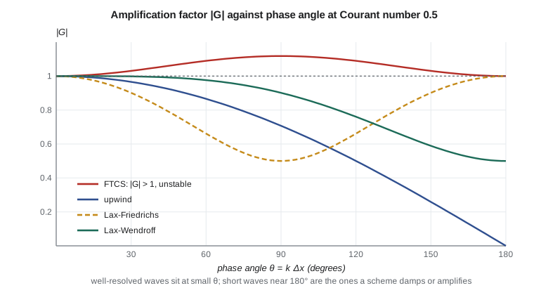
Substituting the mode into the scheme and cancelling common factors gives \(G\) directly. For the upwind scheme, \(u_j^{n+1} = u_j^n - \nu(u_j^n - u_{j-1}^n)\), the substitution gives \(G = 1 - \nu(1 - e^{-\mathrm{i}\theta})\). Its magnitude satisfies \(|G|^{2} = 1 - 2\nu(1 - \nu)(1 - \cos\theta)\), which is at most 1 for every \(\theta\) only if \(0 \le \nu \le 1\). For FTCS, \(G = 1 - \mathrm{i}\nu\sin\theta\), so \(|G|^{2} = 1 + \nu^{2}\sin^{2}\theta\), which exceeds 1 for every nonzero \(\nu\). FTCS amplifies every mode except the longest and the shortest, which is the instability Arjun saw.

# Von Neumann stability analysis of schemes for u_t + a u_x = 0.
# Substitute u_j^n = G^n exp(i j theta) and compute the amplification factor G(theta) for Courant number nu.
import cmath, math
def G(scheme, nu, th):
    e = cmath.exp(1j * th)
    if scheme == "FTCS":           return 1 - 0.5 * nu * (e - 1 / e)
    if scheme == "upwind":         return 1 - nu * (1 - 1 / e)
    if scheme == "Lax-Friedrichs": return 0.5 * (e + 1 / e) - 0.5 * nu * (e - 1 / e)
    if scheme == "Lax-Wendroff":   return 1 - 0.5 * nu * (e - 1 / e) + 0.5 * nu * nu * (e - 2 + 1 / e)
    if scheme == "implicit BTCS":  return 1 / (1 + 0.5 * nu * (e - 1 / e))
thetas = [math.pi * k / 180 for k in range(1, 181)]
print("Largest |G| over all wave numbers")
print("  scheme            nu=0.5    nu=1.0    nu=1.2    nu=5.0")
for s in ("FTCS", "upwind", "Lax-Friedrichs", "Lax-Wendroff", "implicit BTCS"):
    row = [max(abs(G(s, nu, t)) for t in thetas) for nu in (0.5, 1.0, 1.2, 5.0)]
    verdict = "  ".join(f"{g:8.4f}" for g in row)
    print(f"  {s:15s} {verdict}")
print()
# Dissipation and dispersion at nu = 0.5 for a wave resolved by 10 points (theta = 36 degrees)
nu, th = 0.5, math.radians(36)
print("At nu = 0.5, 10 points per wavelength: |G| per step and relative phase speed")
for s in ("upwind", "Lax-Friedrichs", "Lax-Wendroff"):
    g = G(s, nu, th)
    phase = -cmath.phase(g) / (nu * th)          # 1.0 means the wave moves at exactly a
    steps = 10 / nu * 10                         # ten wavelengths of travel
    print(f"  {s:15s} |G| = {abs(g):.4f}, amplitude after 10 wavelengths {abs(g)**steps:.2e}, phase speed ratio {phase:.3f}")
print()
# Diffusion u_t = nu u_xx with FTCS: stable for r = nu dt / dx^2 <= 1/2
print("FTCS for diffusion: G = 1 - 4 r sin^2(theta/2)")
for r in (0.25, 0.5, 0.6):
    print(f"  r = {r:4.2f}: max |G| = {max(abs(1 - 4*r*math.sin(t/2)**2) for t in thetas):.3f}")

Largest |G| over all wave numbers
  scheme            nu=0.5    nu=1.0    nu=1.2    nu=5.0
  FTCS              1.1180    1.4142    1.5620    5.0990
  upwind            1.0000    1.0000    1.4000    9.0000
  Lax-Friedrichs    1.0000    1.0000    1.2000    5.0000
  Lax-Wendroff      1.0000    1.0000    1.8800   49.0000
  implicit BTCS     1.0000    1.0000    1.0000    1.0000

At nu = 0.5, 10 points per wavelength: |G| per step and relative phase speed
  upwind          |G| = 0.9511, amplitude after 10 wavelengths 4.38e-05, phase speed ratio 1.000
  Lax-Friedrichs  |G| = 0.8607, amplitude after 10 wavelengths 9.44e-14, phase speed ratio 1.109
  Lax-Wendroff    |G| = 0.9966, amplitude after 10 wavelengths 5.03e-01, phase speed ratio 0.953

FTCS for diffusion: G = 1 - 4 r sin^2(theta/2)
  r = 0.25: max |G| = 1.000
  r = 0.50: max |G| = 1.000
  r = 0.60: max |G| = 1.400

The first table confirms the theory. Upwind, Lax-Friedrichs and Lax-Wendroff all have \(|G| \le 1\) up to a Courant number of 1 and become unstable above it; at \(\nu = 5\), Lax-Wendroff amplifies the worst mode by a factor of 49 per step. FTCS is unstable at every Courant number. The implicit backward-time central-space scheme, BTCS, has \(|G| \le 1\) for any Courant number: it is unconditionally stable.

The CFL condition

The physical meaning of the Courant number limit was found by Courant, Friedrichs and Lewy in 1928, before stability analysis in its modern form existed. The solution of a hyperbolic equation at a point depends on the initial data within its domain of dependence, the region bounded by the characteristics through that point. An explicit scheme's numerical domain of dependence is the set of grid points its stencil reaches back to. If the physical domain of dependence lies partly outside the numerical one, the scheme ignores data that affect the true solution and cannot converge. For a three-point explicit stencil, this requires the characteristic to travel no more than one cell per step: \(|a|\Delta t/\Delta x \le 1\). The CFL condition is necessary for stability but not sufficient, as FTCS shows: its stencil contains the characteristic, yet it is unstable.

For the Euler equations, the fastest signals move at \(|u| + c\), the flow speed plus the speed of sound. The CFL condition for an explicit Euler solver therefore limits the time step to about \(\Delta t \le \text{CFL} \times \Delta x / (|u| + c)\), where the CFL number is set by the scheme and the time integrator. In a viscous calculation, the smallest cells are in the boundary layer, often a few micrometres thick, and an explicit global time step would be tiny. Steady-state solvers avoid this with local time stepping: each cell advances at its own largest stable step. Since only the final steady state matters, the time accuracy of the path to it is irrelevant.

Dissipation and dispersion

A stable scheme can still be inaccurate. The amplification factor of the exact solution of linear advection has magnitude 1 and phase \(-\nu\theta\): the wave neither grows nor decays and moves exactly at speed \(a\). A numerical scheme has \(|G| < 1\) for some \(\theta\), which is numerical dissipation, and a phase that differs from \(-\nu\theta\), which is dispersion. The second part of the code's output measures both for a wave resolved by 10 points per wavelength, travelling ten wavelengths.

Upwind loses about 5 per cent of the amplitude per step, which compounds to a factor of \(4 \times 10^{-5}\) over 200 steps: the wave is gone. Its phase speed happens to be exact at \(\nu = 0.5\). Lax-Friedrichs is even more dissipative and moves the wave 11 per cent too fast. Lax-Wendroff keeps half the amplitude after ten wavelengths but moves the wave 5 per cent too slowly; after ten wavelengths it lags by half a wavelength. These numbers show why resolution is measured in points per wavelength. For a second-order scheme to carry a wave over long distances, such as a tip vortex traced several spans behind the Petrel 19 for a wake study, needs 20 or more points across the vortex core, and dedicated vortex-tracking studies often use higher-order schemes or adaptive refinement.

Stability of diffusion and of systems

For the diffusion equation with FTCS, \(G = 1 - 4r\sin^{2}(\theta/2)\), where \(r = \nu\Delta t/\Delta x^{2}\). The shortest wave, \(\theta = \pi\), gives \(G = 1 - 4r\), so stability needs \(r \le 1/2\). The code confirms \(|G| = 1.4\) at \(r = 0.6\). For combined advection and diffusion, both limits apply, and for the Navier-Stokes equations the viscous limit usually governs in the boundary layer while the convective limit governs elsewhere. Production codes therefore treat the equations implicitly, or at least the stiffest parts of them.

For a system such as the Euler equations, the amplification factor becomes an amplification matrix, and stability requires its eigenvalues to lie within the unit circle. Von Neumann analysis assumes constant coefficients, periodic boundaries and linearity, none of which hold exactly in a real flow. It is nevertheless a reliable guide: a scheme unstable under von Neumann analysis is almost always unstable in practice, while stability under it is a strong indication, though not a proof, of practical stability. Boundary conditions can add instabilities of their own, which are analysed by other methods.

Time integration for steady and unsteady flow

Most aircraft CFD seeks a steady solution, and the time variable serves only as an iteration parameter. Explicit multistage Runge-Kutta schemes, popularised in Jameson's codes, combine well with local time stepping, residual smoothing and multigrid, which uses a sequence of coarser grids to remove long-wavelength errors that the fine-grid iteration damps slowly. Implicit schemes linearize the residual about the current solution and solve a large sparse system at each iteration, typically with Gauss-Seidel sweeps or a Krylov method such as GMRES. Newton-Krylov solvers can converge in tens of iterations rather than thousands, at the cost of more memory and more care. The Petrel 19 runs use an implicit scheme with a CFL number ramped from 1 to several hundred as the residual falls.

For unsteady flows, such as propeller wakes on the Petrel 19 or buffet on the Swift 900, the time step must resolve the physics. Dual time stepping is the usual approach: each physical time step is solved as a steady problem in a pseudo-time, using all the convergence acceleration of a steady solver, and second-order backward differences in physical time. The physical step is chosen by the time scale of interest, for example a few degrees of propeller rotation, rather than by stability.

Measuring convergence

Iterative convergence is judged by the residual, the amount by which the current solution fails to satisfy the discrete equations, usually reported as a root-mean-square norm over all cells and scaled by its initial value. The group's practice requires the density residual to fall by at least six orders of magnitude and, more importantly, the lift, drag and moment coefficients to settle to within a stated tolerance over the last few hundred iterations. A residual that has fallen four orders while the drag still drifts by a count is not converged. Integrated forces are what the design uses, so they are the final test.