
AERO-440 · Lesson 4 of 12 · 26 min
Finite volume methods
The commercial package the group bought, SU2, OpenFOAM, FUN3D and nearly every other aerodynamic production code share one foundation: the finite-volume method. Tomasz wants the group to understand it from the inside before trusting it with the Swift 900 transonic wing, where the solver must place a shock in the right spot to within a few per cent of chord. Arjun's assignment for this lesson is to write a finite-volume solver for Burgers' equation, the simplest equation that forms shocks, and to find out for himself why the choice of interface flux matters.
Cells, averages and fluxes
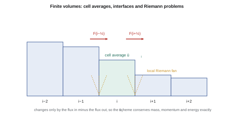
A finite-volume method divides the domain into cells, or control volumes, and stores in each cell the average of the conserved quantity over that cell. The integral form of the conservation law, applied to one cell, says that the average changes only by the fluxes through the cell faces. In one dimension, for cell \(i\) between faces \(i - \tfrac12\) and \(i + \tfrac12\),
This relation is exact if \(F_{i\pm 1/2}\) are the true time-averaged fluxes. The whole art of the method lies in approximating those fluxes from the cell averages on either side. Whatever approximation is chosen, the flux leaving one cell through a face is exactly the flux entering its neighbour. Summing over all cells, the interior fluxes cancel in pairs, and the total of the conserved quantity changes only by the fluxes at the domain boundaries. Mass, momentum and energy are therefore conserved to machine precision, whatever the grid resolution. In three dimensions, the face flux becomes a sum over all the faces of a cell, each weighted by its area, and the cell may be a hexahedron, tetrahedron, prism, pyramid or a general polyhedron. That geometric flexibility is the second great strength of finite volumes.
Godunov's method
Godunov's 1959 idea was to treat the data as piecewise constant: in each cell the solution is exactly its average. At each face there is then a jump between two constant states. A conservation law with a single jump in its initial data is called a Riemann problem, and for many equations, including the Euler equations, its exact solution is known: a fan of waves, shocks, rarefactions and contact surfaces, spreading from the face. Godunov's method evaluates the flux at each face from the exact Riemann solution there and uses it in the finite-volume update. Because the Riemann solution contains the correct physics of wave direction, the method is automatically upwind for systems with waves moving both ways.
For Burgers' equation, the Riemann problem with left state \(u_L\) and right state \(u_R\) has a simple solution. If \(u_L > u_R\), a shock forms, moving at the speed \(s = (u_L + u_R)/2\) given by the jump condition. If \(u_L < u_R\), a rarefaction fan spreads between speeds \(u_L\) and \(u_R\). The Godunov flux is the flux of whatever state sits on the face, at \(x/t = 0\). The one delicate case is the transonic rarefaction, where \(u_L < 0 < u_R\): the face sits inside the fan, at the sonic point where \(u = 0\), and the flux is zero.
Approximate Riemann solvers
Solving the exact Riemann problem for the Euler equations requires an iteration at every face and every step, which was expensive on early computers. Approximate Riemann solvers replace it with something cheaper. Philip Roe's solver of 1981 linearizes the problem about a specially averaged state, so that the jump is decomposed exactly into waves of the linearized system. The Roe flux is
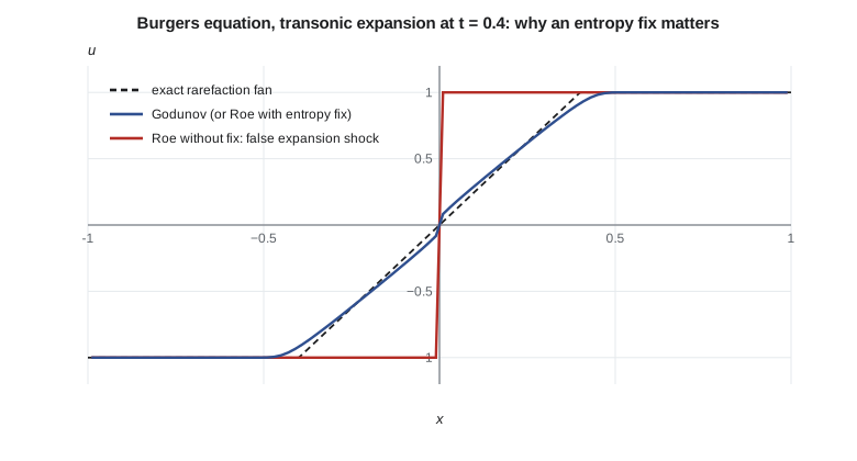
For Burgers' equation, the averaged wave speed is \(\tilde{a} = (u_L + u_R)/2\). The first term is a central average and the second is a dissipation term that upwinds each wave according to the sign of its speed. Roe's solver captures stationary shocks and contact discontinuities exactly, which makes it very accurate for boundary layers, but it has a known flaw. In a transonic rarefaction, the averaged speed can be near zero, the dissipation vanishes, and the scheme can keep an expansion shock: a jump in which the flow accelerates through a discontinuity. Such a shock satisfies the conservation law but violates the entropy condition, the physical requirement that entropy cannot decrease. An entropy fix, such as Harten's, keeps the dissipation from falling to zero inside a fan.
The code below runs three versions on two test cases: a right-moving shock, and a transonic expansion from \(u = -1\) to \(u = 1\) whose exact solution is a fan \(u = x/t\).
# Finite-volume solution of the inviscid Burgers equation u_t + (u^2/2)_x = 0.
# Cell averages are updated by the difference of interface fluxes; three interface fluxes are compared.
def f(u): return 0.5 * u * u
def godunov(ul, ur):                     # exact Riemann solution evaluated at the interface
    if ul > ur:                          # shock, speed (ul + ur) / 2
        return f(ul) if ul + ur > 0 else f(ur)
    if ul > 0: return f(ul)              # rarefaction entirely to the right
    if ur < 0: return f(ur)              # rarefaction entirely to the left
    return 0.0                           # sonic point inside the fan
def roe(ul, ur, fix=False):
    a = 0.5 * (ul + ur)                  # Roe-averaged wave speed for Burgers
    if fix:                              # Harten entropy fix: keep |a| away from zero in a fan
        d = max(0.0, 0.5 * (ur - ul))
        if abs(a) < d: a = (a * a + d * d) / (2 * d)
    return 0.5 * (f(ul) + f(ur)) - 0.5 * abs(a) * (ur - ul)
def solve(flux, ul, ur, n=200, t_end=0.4, cfl=0.8):
    dx = 2.0 / n
    xs = [-1 + (i + 0.5) * dx for i in range(n)]
    u = [ul if x < 0 else ur for x in xs]
    t = 0.0
    while t < t_end - 1e-12:
        dt = min(cfl * dx / max(abs(v) for v in u), t_end - t)
        F = [flux(u[i], u[i + 1]) for i in range(n - 1)]
        u = [u[0]] + [u[i] - dt / dx * (F[i] - F[i - 1]) for i in range(1, n - 1)] + [u[-1]]
        t += dt
    return xs, u
cases = (("shock (1 -> 0)", 1.0, 0.0), ("transonic expansion (-1 -> 1)", -1.0, 1.0))
fluxes = (("Godunov", godunov), ("Roe, no fix", roe), ("Roe + entropy fix", lambda a, b: roe(a, b, True)))
for name, ul, ur in cases:
    print(name, "at t = 0.4")
    for fname, F in fluxes:
        xs, u = solve(F, ul, ur)
        mid = [u[i] for i in range(len(xs)) if abs(xs[i]) < 0.1]
        jump = max(abs(u[i + 1] - u[i]) for i in range(len(u) - 1))
        if ul > ur:
            xs_sh = next(xs[i] for i in range(len(u)) if u[i] < 0.5)
            extra = f"shock at x = {xs_sh:.3f} (exact 0.200)"
        else:
            extra = f"u near x = 0 spans {min(mid):+.3f} to {max(mid):+.3f} (exact fan -0.25 to +0.25)"
        print(f"  {fname:18s} largest cell-to-cell jump {jump:.3f}; {extra}")
    print()
# Conservation check: the total of u*dx changes only by the boundary fluxes
xs, u = solve(godunov, 1.0, 0.0)
print(f"Total u*dx after shock run: {sum(u) * 0.01:.4f} (initial 1.0000 + inflow 0.5*0.4 = 1.2000)")shock (1 -> 0) at t = 0.4 Godunov largest cell-to-cell jump 0.654; shock at x = 0.205 (exact 0.200) Roe, no fix largest cell-to-cell jump 0.654; shock at x = 0.205 (exact 0.200) Roe + entropy fix largest cell-to-cell jump 0.654; shock at x = 0.205 (exact 0.200) transonic expansion (-1 -> 1) at t = 0.4 Godunov largest cell-to-cell jump 0.089; u near x = 0 spans -0.266 to +0.266 (exact fan -0.25 to +0.25) Roe, no fix largest cell-to-cell jump 2.000; u near x = 0 spans -1.000 to +1.000 (exact fan -0.25 to +0.25) Roe + entropy fix largest cell-to-cell jump 0.089; u near x = 0 spans -0.266 to +0.266 (exact fan -0.25 to +0.25) Total u*dx after shock run: 1.2000 (initial 1.0000 + inflow 0.5*0.4 = 1.2000)
All three fluxes place the shock at the right location and keep the total of \(u\) exactly balanced by the boundary fluxes, 1.2000, as the conservation argument predicts. On the expansion, Godunov and the fixed Roe flux reproduce the fan, with the solution near the origin spanning about \(-0.27\) to \(+0.27\) against the exact \(\pm 0.25\); the small excess is first-order smearing. Roe without the fix leaves the initial jump frozen in place: a stationary expansion shock of height 2. This is not a small inaccuracy but a qualitatively wrong flow, and it could appear in a real solver near the sonic line on the Swift 900 wing, where the flow accelerates through Mach 1 near the leading edge.
Other approximate solvers are widely used. The HLL solver of Harten, Lax and van Leer assumes a single intermediate state between the fastest left and right waves; it is robust and positivity-preserving but smears contact surfaces and shear layers. HLLC restores the missing contact wave. Flux-vector splitting methods, such as those of Steger and Warming and of van Leer, split the flux itself into parts carried by right- and left-running waves. The AUSM family of Liou and Steffen treats convective and pressure fluxes separately and is popular for its robustness at all speeds. Lesson 7 applies these to the Euler equations.
Second order: reconstruction and limiters
Godunov's method is first order, with the numerical diffusion of the upwind scheme. To reach second order, the piecewise constant data are replaced by piecewise linear data within each cell: the MUSCL approach of Bram van Leer. A slope is computed for each cell from neighbouring averages, the solution is reconstructed at each side of each face, and the Riemann solver is applied to the two reconstructed values. On smooth data this gives second-order accuracy. Near a jump, the slopes would create new extrema, exactly as Godunov's theorem warns, so the slope is limited.
The limiter function \(\phi(r)\) depends on the ratio of consecutive slopes. Where the solution is smooth, \(r\) is near 1 and \(\phi\) is near 1, giving full second order. At a local extremum or near a jump, \(r\) is negative or extreme and \(\phi\) falls toward zero, reverting to first order. Common limiters include minmod, the most dissipative; van Leer's smooth limiter; and superbee, the least dissipative, which tends to steepen smooth profiles into square ones. Limiters with these properties make the scheme total-variation diminishing, or TVD: the sum of the absolute jumps between neighbouring cells cannot grow. The price is that TVD schemes drop to first order at smooth extrema, clipping peaks slightly.
Limiters can also stall convergence. In a steady calculation, a limiter that switches back and forth between iterations near a shock can keep the residual from falling below a certain level. Practical solvers use smooth limiters, or freeze the limiter after the residual has dropped by a few orders of magnitude. When a solver's convergence history levels off at a plateau with a noisy limit cycle, the limiter is the first suspect.
Unstructured finite volumes
On an unstructured grid of tetrahedra, prisms and other shapes, the same principles apply. Two arrangements are common. In a cell-centred scheme, the unknowns live at the cell centroids and the control volumes are the cells themselves. In a vertex-centred scheme, the unknowns live at the grid nodes and each node has a dual control volume built from parts of the surrounding cells; FUN3D and SU2 use this arrangement. Gradients for reconstruction are found by least squares or by the Green-Gauss theorem from the neighbouring values. On highly stretched boundary-layer cells, the choice of gradient method has a measurable effect on accuracy, and solver documentation usually recommends weighted least squares for such grids.
| Flux or method | Strength | Weakness |
|---|---|---|
| Exact Riemann (Godunov) | Correct physics, sharp shocks | Expensive iteration at every face |
| Roe | Exact contacts and shear layers; accurate boundary layers | Needs an entropy fix; can fail at strong expansions |
| HLL | Very robust; keeps density and pressure positive | Smears contacts and shear layers |
| HLLC | Robust and resolves contacts | Slightly more complex than HLL |
| AUSM family | Robust, good at low and high speeds | Some variants need tuning near walls |
| Central with artificial dissipation | Simple and cheap | Dissipation coefficients must be tuned |
Worked problem
Shock speed from the jump condition
A Burgers' shock has \(u_L = 1\) and \(u_R = 0\). Where is it at \(t = 0.4\) if it starts at \(x = 0\)?
Show solution
- The jump condition gives \(s = [f]/[u] = (\tfrac12 - 0)/(1 - 0) = 0.5\).
- Position \(= s\,t = 0.5 \times 0.4 = 0.2\).
Answer: At \(x = 0.2\), as the code found.
Worked problem
Conservation check
In the shock run, the domain runs from \(-1\) to 1 and initially \(u = 1\) for \(x < 0\). The left boundary keeps \(u = 1\). What should the total of \(u\,\Delta x\) be at \(t = 0.4\)?
Show solution
- Initial total: \(1 \times 1 = 1.0\).
- Flux in at the left: \(f(1) = 0.5\) per unit time; flux out at the right: \(f(0) = 0\).
- Change: \(0.5 \times 0.4 = 0.2\).
Answer: 1.2, matched exactly by the code because the scheme is conservative.
Worked problem
Limiter behaviour at an extremum
Three consecutive cell averages are 0.8, 1.0 and 0.9, so cell 2 is a local maximum. What slope does a TVD limiter give cell 2, and why?
Show solution
- Backward difference: \(1.0 - 0.8 = 0.2\); forward difference: \(0.9 - 1.0 = -0.1\).
- Ratio \(r = -0.1/0.2 = -0.5\), negative at an extremum.
- TVD limiters set \(\phi(r) = 0\) for \(r \le 0\).
Answer: Zero slope. The scheme drops to first order at the peak, which is why TVD schemes slightly clip smooth maxima.
Common mistakes
MistakeAny flux that is consistent will give the right answer at shocks.
InsteadFluxes without enough dissipation in expansions can keep entropy-violating expansion shocks.
MistakeFinite volumes conserve mass only on fine grids.
InsteadConservation is exact on any grid because each face flux is shared by its two cells.
MistakeLimiters only affect solutions with shocks.
InsteadLimiters also act at smooth extrema and can stall steady convergence anywhere they switch.
MistakeHLL is best because it is most robust.
InsteadHLL smears contacts and shear layers, which harms boundary-layer accuracy; HLLC or Roe is usually preferred for viscous flows.
Summary and key terms
- The finite-volume method stores cell averages and updates them by the difference of face fluxes, which conserves mass, momentum and energy exactly on any grid.
- Godunov's method takes each face flux from a Riemann problem and is naturally upwind.
- Approximate Riemann solvers such as Roe, HLL, HLLC and AUSM reduce the cost; Roe needs an entropy fix to avoid expansion shocks.
- MUSCL reconstruction with slope limiters gives second order in smooth regions while avoiding oscillations at jumps.
- Unstructured solvers apply the same ideas on cell-centred or vertex-centred control volumes.
- Control volume
- A cell over which the integral conservation law is applied.
- Riemann problem
- A conservation law with initial data consisting of two constant states separated by a jump.
- Roe solver
- An approximate Riemann solver based on a linearization about an averaged state.
- Entropy fix
- A modification that keeps an upwind flux from admitting expansion shocks.
- MUSCL
- Piecewise linear reconstruction within cells to reach second-order accuracy.
- Limiter
- A function that reduces reconstructed slopes near extrema and discontinuities.
- TVD
- Total-variation diminishing: the sum of absolute jumps between cells cannot grow.
Practice problems
Work each problem on paper first, then reveal the answer to check.
What is the Godunov flux for Burgers' equation when \(u_L = -0.5\) and \(u_R = 0.8\)?
Show answer
A transonic rarefaction: the face sees \(u = 0\), so the flux is 0.
What is the Godunov flux when \(u_L = 2\) and \(u_R = 1\)?
Show answer
A shock moving right at 1.5; the face sees \(u_L\), so the flux is \(2^2/2 = 2\).
Why is a stationary expansion shock unphysical?
Show answer
Entropy would decrease through it, violating the second law.
Which limiter is the most dissipative of minmod, van Leer and superbee?
Show answer
Minmod.
Name the two arrangements of unknowns in unstructured finite-volume codes.
Show answer
Cell-centred and vertex-centred.
Lesson quiz · 5 questions
Score 60% or more to complete this lesson.
Create a free account to save your progress, take quizzes and earn a certificate.