Panel methods

Thin airfoil theory treats every section as if it had no thickness. To predict the pressure on the real surface of the NACA 4415, including the suction peak at the nose that controls the stall, Arjun needs a method that represents the actual shape. Panel methods do exactly that. They cover the surface with flat panels, put a simple singularity on each one, and solve a set of linear equations so that no flow passes through any panel. Developed at Douglas Aircraft in the 1960s by John Hess and A. M. O. Smith, panel methods were the first computer methods to change how aircraft were designed, and they remain the fastest way to analyse the inviscid flow around a complicated shape.

The idea: singularities on the surface

Lesson 3 built a Rankine oval from a source and a sink placed inside the body, and found the body shape that resulted. Design needs the opposite: start from a given shape and find the singularities that produce it. A panel method spreads singularities over the surface itself. The surface is divided into \(N\) straight panels. Each panel carries a source distribution of constant strength \(\lambda_j\) and, for a lifting body, a vortex distribution. The velocity at any point is the free stream plus the sum of the contributions of all panels. Each panel's contribution is proportional to its unknown strength, multiplied by an influence coefficient that depends only on geometry.

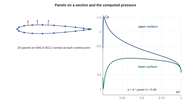
The boundary condition is applied at one control point on each panel, usually its midpoint: the velocity normal to the panel must be zero. That gives \(N\) linear equations. For a lifting airfoil the Hess-Smith formulation uses a single vortex strength \(\gamma\), the same on every panel, as one extra unknown, and adds one extra equation: the Kutta condition, written as equal tangential speeds on the two panels that meet at the trailing edge, so that the flow leaves smoothly. Solving the \(N + 1\) equations gives all the strengths, after which the tangential velocity at every control point, and hence the pressure coefficient, follows directly.

Influence coefficients

The influence of a constant-strength source panel on a point can be integrated exactly. The velocity it induces involves two geometric quantities: the logarithm of the ratio of the distances from the point to the panel's two ends, and the angle the panel subtends at the point. A constant-strength vortex panel induces the same two quantities with their roles rotated by 90 degrees. On its own control point, a source panel induces a normal velocity of exactly half its strength and no tangential velocity, which is why the diagonal of the source matrix is one half. The program uses these exact formulas.

The computing cost is dominated by solving the linear system. With direct Gaussian elimination it grows with the cube of the number of panels, so 80 panels cost about eight times as much as 40. In two dimensions this is trivial: a section with 200 panels is solved in a fraction of a second. In three dimensions a whole aircraft may need tens of thousands of panels, and iterative solvers and clever ways of grouping distant panels are used.

# A vortex panel method (Hess-Smith: constant sources plus one vortex) for a NACA four-digit section
import math
def naca4(code, n):                        # surface points from trailing edge, over the lower then upper surface
    m, p, t = int(code[0]) / 100, int(code[1]) / 10, int(code[2:]) / 100
    up, lo = [], []
    for i in range(n + 1):
        x = 0.5 * (1 - math.cos(math.pi * i / n))
        yt = 5 * t * (0.2969 * math.sqrt(x) - 0.1260 * x - 0.3516 * x**2 + 0.2843 * x**3 - 0.1036 * x**4)
        if m == 0: yc, dy = 0.0, 0.0
        elif x < p: yc, dy = m / p**2 * (2 * p * x - x * x), 2 * m / p**2 * (p - x)
        else: yc, dy = m / (1 - p)**2 * ((1 - 2 * p) + 2 * p * x - x * x), 2 * m / (1 - p)**2 * (p - x)
        th = math.atan(dy)
        up.append((x - yt * math.sin(th), yc + yt * math.cos(th))); lo.append((x + yt * math.sin(th), yc - yt * math.cos(th)))
    return lo[::-1] + up[1:]
def solve(A, b):                           # Gaussian elimination with partial pivoting
    n = len(b); M = [row[:] + [b[i]] for i, row in enumerate(A)]
    for k in range(n):
        piv = max(range(k, n), key=lambda r: abs(M[r][k])); M[k], M[piv] = M[piv], M[k]
        for r in range(k + 1, n):
            f = M[r][k] / M[k][k]
            for c in range(k, n + 1): M[r][c] -= f * M[k][c]
    x = [0.0] * n
    for k in range(n - 1, -1, -1):
        x[k] = (M[k][n] - sum(M[k][c] * x[c] for c in range(k + 1, n))) / M[k][k]
    return x
def hess_smith(code, alpha_deg, n=40):
    P = naca4(code, n); N = len(P) - 1; al = math.radians(alpha_deg)
    th = [math.atan2(P[j + 1][1] - P[j][1], P[j + 1][0] - P[j][0]) for j in range(N)]
    mid = [((P[j][0] + P[j + 1][0]) / 2, (P[j][1] + P[j + 1][1]) / 2) for j in range(N)]
    ln = [math.hypot(P[j + 1][0] - P[j][0], P[j + 1][1] - P[j][1]) for j in range(N)]
    def infl(i, j):                        # normal and tangential velocity at mid i from unit source on panel j
        if i == j: return 0.5, 0.0, 0.0, 0.5
        r1 = math.hypot(mid[i][0] - P[j][0], mid[i][1] - P[j][1]); r2 = math.hypot(mid[i][0] - P[j + 1][0], mid[i][1] - P[j + 1][1])
        b = math.atan2((mid[i][1] - P[j + 1][1]) * (mid[i][0] - P[j][0]) - (mid[i][0] - P[j + 1][0]) * (mid[i][1] - P[j][1]),
                       (mid[i][0] - P[j + 1][0]) * (mid[i][0] - P[j][0]) + (mid[i][1] - P[j + 1][1]) * (mid[i][1] - P[j][1]))
        lr = math.log(r2 / r1); d = th[i] - th[j]
        sn = (math.sin(d) * lr + math.cos(d) * b) / (2 * math.pi); st = (math.sin(d) * b - math.cos(d) * lr) / (2 * math.pi)
        return sn, st, -st, sn                 # source normal, source tangential, vortex normal, vortex tangential
    A = [[0.0] * (N + 1) for _ in range(N + 1)]; rhs = [0.0] * (N + 1); T = [[0.0] * (N + 1) for _ in range(N)]
    for i in range(N):
        for j in range(N):
            sn, st, vn, vt = infl(i, j)
            A[i][j] = sn; A[i][N] += vn; T[i][j] = st; T[i][N] += vt
        rhs[i] = -math.sin(al - th[i])
    for j in range(N + 1):                 # Kutta condition: equal tangential speeds at the two trailing-edge panels
        A[N][j] = T[0][j] + T[N - 1][j]
    rhs[N] = -math.cos(al - th[0]) - math.cos(al - th[N - 1])
    x = solve(A, rhs)
    vt = [sum(T[i][j] * x[j] for j in range(N + 1)) + math.cos(al - th[i]) for i in range(N)]
    cp = [1 - v * v for v in vt]
    cl = -sum(cp[i] * ln[i] * math.cos(th[i] - al) for i in range(N))   # lift from the surface pressures
    return cl, min(cp), mid, cp
for code, a in (('0012', 0), ('0012', 4), ('0012', 8), ('4415', 0), ('4415', 4)):
    cl, cpmin, mid, cp = hess_smith(code, a)
    thin = 2 * math.pi * math.radians(a) if code == '0012' else 2 * math.pi * (math.radians(a) + math.radians(4.15))
    print(f"NACA {code} at {a} deg: panel cl = {cl:.3f}, thin-airfoil cl = {thin:.3f}, Cp,min = {cpmin:.2f}")
for n in (10, 20, 40, 80):
    print(f"NACA 0012 at 4 deg with {2 * n} panels: cl = {hess_smith('0012', 4, n)[0]:.4f}")

NACA 0012 at 0 deg: panel cl = 0.000, thin-airfoil cl = 0.000, Cp,min = -0.41
NACA 0012 at 4 deg: panel cl = 0.482, thin-airfoil cl = 0.439, Cp,min = -1.52
NACA 0012 at 8 deg: panel cl = 0.961, thin-airfoil cl = 0.877, Cp,min = -4.22
NACA 4415 at 0 deg: panel cl = 0.520, thin-airfoil cl = 0.455, Cp,min = -0.89
NACA 4415 at 4 deg: panel cl = 1.011, thin-airfoil cl = 0.894, Cp,min = -1.44
NACA 0012 at 4 deg with 20 panels: cl = 0.4835
NACA 0012 at 4 deg with 40 panels: cl = 0.4810
NACA 0012 at 4 deg with 80 panels: cl = 0.4818
NACA 0012 at 4 deg with 160 panels: cl = 0.4822

What the panel method shows

For the symmetrical NACA 0012 at zero angle of attack the program correctly finds no lift, and a minimum pressure coefficient of minus 0.41 at about the point of maximum thickness: the thickness alone speeds up the flow, as on the Rankine oval. At 4 degrees the lift coefficient is 0.482, about 10 percent above the thin-airfoil value of 0.439. That difference is real for inviscid flow: thickness raises the lift slope slightly, as the Joukowski result in Lesson 4 suggested. Measured lift coefficients for the 0012 at 4 degrees are close to 0.43 to 0.44, a little below even thin airfoil theory, because the real boundary layer reduces the effective camber near the trailing edge. A panel method alone therefore overpredicts lift slightly; coupling it with a boundary-layer calculation, as viscous-inviscid programs do, brings it into line.

The pressure distribution is the most valuable output. At 8 degrees the suction peak on the NACA 0012 reaches a pressure coefficient of about minus 4.2, very close to the nose. Such a sharp peak followed by a steep pressure rise is the warning sign of leading-edge stall: the boundary layer must climb a large pressure hill in a short distance. For the cambered NACA 4415, camber spreads the lift over more of the chord, so at 4 degrees, where it produces about twice the lift of the 0012, its suction peak is only minus 1.44 against minus 1.52. This is the key reason cambered, thicker sections reach higher maximum lift: they make lift with gentler peaks.

The convergence check at the end is a habit every engineer using a numerical method should have. With 20 panels the lift coefficient is 0.4835; with 40, 80 and 160 it settles at about 0.482. The lift converges quickly, but the peak suction near the nose needs more panels to resolve, because it is a sharp feature. Professional practice is to repeat the calculation with more panels until the quantity of interest stops changing by more than the accuracy needed.

Panel methods in three dimensions and in industry

Three-dimensional panel methods cover a complete aircraft surface with quadrilateral panels carrying sources and doublets, and shed a sheet of doublets from wing trailing edges to represent the wake. They predict the lift distribution along the span, the interference between wing and fuselage, the pressures on nacelles and the effect of the tail. Programs of this kind, many developed in the 1970s and 1980s by aircraft companies and by the National Research Council, remain standard for early design, for loads and for flight simulator data because they run in seconds or minutes rather than the hours or days needed for full viscous simulations.

Their limits follow from the potential-flow assumption. A panel method knows nothing of the boundary layer, so it cannot predict drag other than induced drag, cannot predict separation, and loses accuracy wherever the boundary layer is thick or the flow is separated: near the stall, behind flap gaps and on bluff parts of the fuselage. It also assumes incompressible flow unless a compressibility correction is applied. AERO-440 introduces the computational fluid dynamics methods that solve the Euler and Navier-Stokes equations directly and overcome these limits at much higher cost.

Using panel results on the Block 2 wing

Tomasz's group ran a three-dimensional panel model of the Block 2 wing and fuselage early in the design. It confirmed the lifting-line predictions of Lesson 9 for the spanwise lift distribution, showed that the fuselage carries a modest share of the lift and that the lift is reduced in the wing-fuselage junction, and gave the pressures the loads team needed for the first structural sizing. For the stall work the team switched to the wind tunnel and to viscous computations, because the panel method cannot predict where the flow will separate. Arjun's job was to run the two-dimensional program on each candidate section and plot the pressure distributions at the approach lift coefficient, flagging any with suction peaks steep enough to worry about.