
AERO-300 · Lesson 3 of 12 · 24 min
Potential flow and elementary flows
Lesson 2 showed that the air outside the boundary layer and wake of a wing is essentially irrotational. That single fact transforms the mathematics. An irrotational velocity field can be written as the gradient of a scalar function, the velocity potential, and in incompressible flow that potential obeys Laplace's equation, which is linear. Linear equations allow superposition: simple solutions can be added to build complicated ones. In this lesson Arjun learns the handful of elementary flows from which panel methods, thin airfoil theory and lifting-line theory are all assembled. Students who have taken Fluid Mechanics II will recognize the building blocks; here we use them as an aerodynamicist does, with an eye to representing wings.
The velocity potential and Laplace's equation
If the vorticity is zero, \(\nabla\times\mathbf{V} = 0\), and a standard vector identity says the velocity must be the gradient of some scalar \(\phi\). That scalar is the velocity potential. Substituting \(\mathbf{V} = \nabla\phi\) into the incompressible continuity equation \(\nabla\cdot\mathbf{V} = 0\) gives Laplace's equation.
Laplace's equation is one of the most studied equations in physics: it also governs steady heat conduction, electrostatics and groundwater flow. Its solutions are smooth inside the flow and are fixed completely by conditions on the boundaries. For flow around a body, the boundary conditions are that the flow becomes the uniform free stream far away and that no fluid passes through the body surface. Once \(\phi\) is known, the velocity follows by differentiation and the pressure follows from Bernoulli's equation. The momentum equation never has to be solved directly.
Because Laplace's equation is linear, the sum of any two solutions is also a solution. That is the principle of superposition, and it makes potential flow a construction kit: find a few simple solutions, then add them with the right strengths and positions so that the combination satisfies the boundary conditions for the body of interest.
The stream function
In two-dimensional incompressible flow there is a second useful function, the stream function \(\psi\), defined so that continuity is satisfied automatically. Lines of constant \(\psi\) are streamlines, and the difference in \(\psi\) between two streamlines equals the volume flow rate per unit depth between them. Where streamlines crowd together the flow is fast; where they spread apart it is slow.
For irrotational flow, \(\psi\) also satisfies Laplace's equation. Lines of constant \(\phi\), called equipotential lines, cross the streamlines at right angles everywhere except at stagnation points. The most useful property of \(\psi\) for aerodynamics is that any streamline can be replaced by a solid surface without changing the flow, since no fluid crosses a streamline. So if we can find a superposition in which one closed streamline has the shape we want, we have found the flow around that shape.
The elementary flows
Four elementary flows are enough for almost everything in this course. Their potentials and stream functions are listed below in polar coordinates \((r, \theta)\) centred on the singularity, with the uniform stream along the x axis.
| Flow | Velocity potential φ | Stream function ψ | Velocity |
|---|---|---|---|
| Uniform stream | \(V_\infty r\cos\theta\) | \(V_\infty r\sin\theta\) | \(V_\infty\) in the x direction |
| Source of strength Λ | \(\frac{\Lambda}{2\pi}\ln r\) | \(\frac{\Lambda}{2\pi}\theta\) | radial, \(V_r = \Lambda/(2\pi r)\) |
| Vortex of strength Γ | \(-\frac{\Gamma}{2\pi}\theta\) | \(\frac{\Gamma}{2\pi}\ln r\) | circular, \(V_\theta = -\Gamma/(2\pi r)\) |
| Doublet of strength κ | \(\frac{\kappa}{2\pi}\frac{\cos\theta}{r}\) | \(-\frac{\kappa}{2\pi}\frac{\sin\theta}{r}\) | loops leaving and returning to the origin |
A source emits fluid equally in all directions; its strength \(\Lambda\) is the volume flow rate per unit depth, and a negative source is a sink. The vortex is the free vortex of Lesson 2, with circulation \(\Gamma\) around any curve enclosing it. A doublet is the limit of a source and a sink of equal strength brought together while the product of strength and spacing is held constant; its streamlines are circles tangent to the x axis at the origin. Each elementary flow has a singular point where the speed becomes infinite. In a model of a real body those points are always placed inside the body, where the flow is not real anyway.
Building bodies by superposition
Adding a source to a uniform stream gives the Rankine half-body: the fluid from the source is pushed downstream by the stream and forms a blunt-nosed body that extends to infinity downstream. The stagnation point sits a distance \(\Lambda/(2\pi V_\infty)\) upstream of the source, and far downstream the body has a width \(\Lambda/V_\infty\), just wide enough to carry the source's flow at free-stream speed.
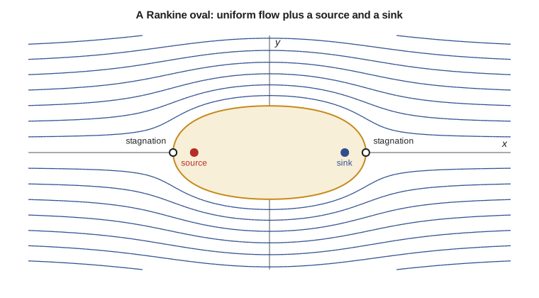
Adding a sink of equal strength downstream of the source closes the body. The result is the Rankine oval, a closed, symmetrical body whose length and thickness depend on the source strength and spacing. The program in this lesson builds a Rankine oval using a convenient tool, the complex potential, and finds its stagnation points, thickness and peak surface speed.
The complex potential
In two dimensions, \(\phi\) and \(\psi\) can be combined into one complex function, the complex potential \(W = \phi + i\psi\), of the complex variable \(z = x + iy\). Its derivative gives the velocity in a compact form, \(dW/dz = u - iv\). Every analytic function of \(z\) is automatically a potential flow, and the elementary flows become very simple expressions: the uniform stream is \(V_\infty z\), a source is \((\Lambda/2\pi)\ln z\), and a clockwise vortex is \((i\Gamma/2\pi)\ln z\). Superposition is just addition.
Complex variables are not needed to use panel methods, but they underpin the conformal mapping methods that were the main tool of airfoil theory for half a century. The Joukowski transformation, \(\zeta = z + R^2/z\), maps a circle into a family of airfoil-like shapes with a sharp trailing edge, so the exact flow past those Joukowski airfoils follows from the flow past a cylinder, which Lesson 4 develops.
# Superposition with the complex potential: a Rankine oval in uniform flow
import cmath, math
Vinf, m, a = 30.0, 60.0, 1.0           # free stream m/s, source strength m2/s, source/sink half spacing m
def w_dot(z):                          # complex velocity dW/dz = u - i v
    return Vinf + m / (2 * math.pi) * (1 / (z + a) - 1 / (z - a))
def psi(z):                            # stream function
    return Vinf * z.imag + m / (2 * math.pi) * (cmath.phase(z + a) - cmath.phase(z - a))
# stagnation points on the x axis: u = 0
L = a * math.sqrt(1 + m / (math.pi * Vinf * a))
print(f"Stagnation points at x = +/-{L:.3f} m (oval length {2 * L:.3f} m)")
print(f"Check: speed at stagnation point = {abs(w_dot(complex(L, 0))):.2e} m/s")
# half thickness h solves h = (m/(2 pi Vinf)) * 2 atan(2 a h/(h^2 - a^2 ... )) -> bisection on psi = 0
lo, hi = 1e-3, 5.0
for _ in range(60):
    mid = (lo + hi) / 2
    if psi(complex(0, mid)) > 0: hi = mid
    else: lo = mid
print(f"Half thickness {lo:.3f} m, thickness ratio {2 * lo / (2 * L):.3f}")
umax = w_dot(complex(0, lo)).real
print(f"Maximum surface speed {umax:.1f} m/s, Cp,min = {1 - (umax / Vinf) ** 2:.3f}")
for x in (-1.5, -0.5, 0.5, 1.5):
    wv = w_dot(complex(x, 1.0))
print(f"point ({x:4.1f}, 1.0): u = {wv.real:6.2f} v = {-wv.imag:6.2f} m/s")Stagnation points at x = +/-1.279 m (oval length 2.559 m) Check: speed at stagnation point = 0.00e+00 m/s Half thickness 0.638 m, thickness ratio 0.499 Maximum surface speed 43.6 m/s, Cp,min = -1.109 point (-1.5, 1.0): u = 29.47 v = 6.32 m/s point (-0.5, 1.0): u = 38.23 v = 4.70 m/s point ( 0.5, 1.0): u = 38.23 v = -4.70 m/s point ( 1.5, 1.0): u = 29.47 v = -6.32 m/s
With a source of 60 m²/s at 1 m from the origin in a 30 m/s stream, the oval is 2.56 m long and 1.28 m thick, a thickness ratio of about one half. The maximum surface speed, at the shoulders, is 43.6 m/s, giving \(C_p = -1.11\). The velocities above the body show the symmetry of the flow: the vertical component reverses sign between the front and rear halves, and the pressure distribution is symmetrical front to back. That symmetry has an important consequence: the net force on the oval is zero. Inviscid potential flow predicts no drag on any closed two-dimensional body without circulation, a result called d'Alembert's paradox, discussed in Lesson 4.
Uniqueness and the role of circulation
For a body in a uniform stream, the flow that satisfies Laplace's equation, the no-penetration condition on the surface and the free-stream condition far away is unique up to one thing: the circulation around the body. Any amount of circulation can be added, because a vortex placed inside the body satisfies Laplace's equation, has no normal velocity on a circle around it and dies away far from the body. For a symmetrical body like the oval at zero incidence the physically sensible choice is zero circulation. For an airfoil, Lesson 2 showed that the Kutta condition picks the value. Every method in the next lessons, from thin airfoil theory to panel methods to lifting-line theory, therefore has two ingredients: singularities that represent the body's thickness and camber, and a vortex distribution whose total strength is set by the Kutta condition.
It is worth pausing on how much potential flow can and cannot do. It predicts surface pressures, and therefore lift and pitching moment, very well for attached flow at moderate angles of attack. It predicts no drag at all in two dimensions and only induced drag in three. It cannot predict separation or stall. Those limits are why aerodynamicists couple potential-flow methods with boundary-layer calculations, the approach behind widely used airfoil design programs.
Worked problem
Sizing a Rankine half-body nose
Tomasz wants a smooth, blunt fairing for a probe mount whose downstream width must be 0.20 m. Model it as a Rankine half-body in a 50 m/s stream. Find the source strength and how far ahead of the source the stagnation point lies.
Show solution
- Far downstream the half-body width is \(h = \Lambda/V_\infty\), so \(\Lambda = 0.20\times 50 = 10\ \text{m}^2/\text{s}\).
- The stagnation point is at \(x_s = -\Lambda/(2\pi V_\infty) = -10/(2\pi\times 50) = -0.0318\ \text{m}\).
Answer: The source sits 32 mm behind the nose. A designer can now place the fairing's nose and know the pressure distribution over it exactly, at least while the flow stays attached.
Worked problem
Speed over the shoulder of the oval
Using the program's oval, find the pressure difference between the free stream and the shoulder at sea level, and say what would happen if the source strength were doubled.
Show solution
- \(q_\infty = 0.5\times 1.225\times 30^2 = 551\ \text{Pa}\).
- \(p - p_\infty = C_p q_\infty = -1.109\times 551 = -611\ \text{Pa}\).
- Doubling \(\Lambda\) makes the oval fatter relative to its length, so the flow must accelerate more over the shoulder and the suction rises.
Answer: Thicker bodies produce stronger suction peaks and, in a real fluid, steeper adverse pressure gradients behind the shoulder, which promote separation. The same trade appears in airfoil thickness in Lesson 5.
Common mistakes
MistakeUsing the velocity potential for a flow that has vorticity.
InsteadA velocity potential exists only where the flow is irrotational. Inside boundary layers and wakes it does not apply.
MistakeForgetting that superposition works for φ and ψ but not directly for pressure.
InsteadVelocities add, but pressure depends on the square of speed. Add the potentials or velocities first, then use Bernoulli's equation.
MistakePlacing a singularity outside the body being modelled.
InsteadSources, sinks, vortices and doublets have infinite speeds at their centres. They must sit inside the body or on its surface in a way that is integrated properly.
MistakeExpecting potential flow to predict drag on a closed two-dimensional body.
InsteadIt predicts zero drag, which is d'Alembert's paradox. Drag comes from viscous effects that potential flow omits.
Summary and key terms
- Irrotational, incompressible flow can be described by a velocity potential φ satisfying Laplace's equation.
- In two dimensions a stream function ψ also exists, and its contours are streamlines.
- Because Laplace's equation is linear, elementary flows such as the uniform stream, source, sink, vortex and doublet can be superposed to model bodies, with any closed streamline treated as a solid surface.
- The complex potential packages φ and ψ together.
- The solution for a body is unique except for the circulation, which the Kutta condition fixes for an airfoil.
- Velocity potential
- A scalar function whose gradient is the velocity in an irrotational flow.
- Stream function
- A function whose contours are streamlines in two-dimensional incompressible flow.
- Laplace's equation
- The linear equation ∇²φ = 0 satisfied by the potential of incompressible irrotational flow.
- Superposition
- Adding solutions of a linear equation to form a new solution.
- Source
- An elementary flow emitting fluid radially from a point.
- Doublet
- The limit of a source and sink brought together with constant strength times spacing.
- Rankine oval
- A closed body formed by a uniform stream, a source and an equal sink.
- Complex potential
- The complex function W = φ + iψ whose derivative gives u − iv.
Practice problems
Work each problem on paper first, then reveal the answer to check.
Show that φ = x² − y² satisfies Laplace's equation and find the velocity at (1, 2).
Show answer
∂²φ/∂x² + ∂²φ/∂y² = 2 − 2 = 0. u = 2x = 2, v = −2y = −4.
A source of strength 6 m²/s is placed in a 12 m/s stream. Find the half-body's width far downstream and the stagnation point position.
Show answer
Width Λ/V = 0.5 m; stagnation point 6/(2π × 12) = 0.080 m upstream of the source.
What is the speed at a distance of 0.5 m from a vortex of strength 3 m²/s?
Show answer
V = Γ/(2πr) = 3/(2π × 0.5) = 0.95 m/s.
Why can a streamline be replaced by a solid wall in potential flow?
Show answer
No fluid crosses a streamline, so a wall along it satisfies the no-penetration condition and leaves the inviscid flow unchanged.
In the program, halve the source strength. What happens to the oval's length and thickness ratio?
Show answer
Both shrink: L = a√(1 + Λ/(πV a)) falls to about 1.15 m, and the thickness ratio drops to about 0.33.
Write the complex potential of a uniform stream plus a clockwise vortex of strength Γ at the origin.
Show answer
W = V∞ z + (iΓ/2π) ln z.
Lesson quiz · 5 questions
Score 60% or more to complete this lesson.
Create a free account to save your progress, take quizzes and earn a certificate.