
NUC-310 · Lesson 5 of 12 · 19 min
Gamma spectroscopy
On a Monday morning a drum of spent resin from the station's purification system arrives at the counting room for waste characterization. Before it can be shipped, the radionuclides in it must be identified and their activities estimated. Marcel asks Hana to run the germanium spectrum and walk him through every feature on it. Reading a gamma spectrum is a core skill for anyone who works with radiation, and it starts with understanding how a single gamma ray deposits its energy in a detector.
How gamma rays deposit energy
A gamma ray interacts in a detector by three main processes. In the photoelectric effect, the photon is absorbed by an atom and an electron is ejected carrying almost all its energy; the atom's X-ray or Auger emission usually deposits the rest locally. In Compton scattering, the photon gives part of its energy to an electron and continues at a lower energy in a new direction. In pair production, which is possible only above 1022 keV, the photon converts into an electron and a positron in the field of a nucleus; the positron later annihilates, producing two 511 keV photons.
The photoelectric effect dominates at low energy and in high atomic number materials, Compton scattering dominates in the middle range from a few hundred keV to several MeV, and pair production becomes important at high energy. A detector records the total energy deposited by all the electrons a photon sets in motion. If every bit of the photon's energy stays in the crystal, through a photoelectric absorption or a chain of Compton scatters ending in one, the event lands in the full-energy peak, or photopeak. If part of the energy escapes, the event lands somewhere lower.
Features of a gamma spectrum
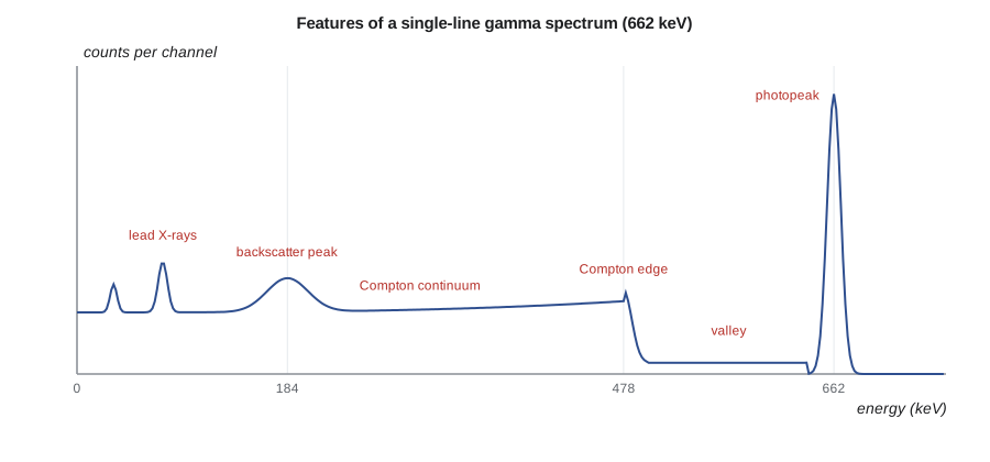
For a photon of energy \(E\) that Compton scatters once and escapes, the electron's energy depends on the scattering angle. The maximum, for a photon scattered straight back, defines the Compton edge:
where \(m_e c^2 = 511\) keV. Below the edge, the Compton continuum extends down to near zero. Between the edge and the photopeak lies a valley that is filled partly by multiple Compton scattering. A backscatter peak appears at \(E - E_{\text{edge}}\), around 200 keV for most energies, from photons that scatter backward in the shield or surrounding material and are then absorbed in the detector. Lead shields also produce characteristic lead X-rays near 75 and 85 keV, which is why shields are lined with cadmium and copper.
Above 1022 keV, pair production adds two more features. If one annihilation photon escapes, the event appears in a single-escape peak at \(E - 511\) keV; if both escape, in a double-escape peak at \(E - 1022\) keV. A 511 keV annihilation peak may also appear from positrons created in the surroundings. When two gamma rays from one decay are detected together, a sum peak appears at their combined energy, as noted for cobalt-60 in lesson 4.
# Gamma spectroscopy: Compton edge, net peak area and activity from a calibrated efficiency.
import math
me = 511.0
for E in (662.0, 1173.2, 1332.5):
    edge = E * (2 * E / me) / (1 + 2 * E / me)
    back = E - edge
    print(f"{E:7.1f} keV: Compton edge {edge:6.1f} keV, backscatter peak {back:5.1f} keV")

# Net peak area with a linear background from regions either side of the peak
roi = 15840            # counts in peak region (n channels)
n = 20
left, right, m = 1210, 1150, 10   # counts in m channels each side
B = n * (left + right) / (2 * m)
net = roi - B
sig = math.sqrt(roi + (n / (2 * m))**2 * (left + right))
print(f"\nbackground under peak {B:.0f}, net area {net:.0f} +/- {sig:.0f} counts")

# Activity of Cs-137 in a sample: A = N / (eff * yield * t)
eff, y, t = 0.0215, 0.851, 3600.0
A = net / (eff * y * t)
print(f"activity {A:.1f} Bq (+/- {A*sig/net:.1f} Bq counting only)")662.0 keV: Compton edge 477.7 keV, backscatter peak 184.3 keV 1173.2 keV: Compton edge 963.4 keV, backscatter peak 209.8 keV 1332.5 keV: Compton edge 1118.1 keV, backscatter peak 214.4 keV background under peak 2360, net area 13480 +/- 135 counts activity 204.7 Bq (+/- 2.0 Bq counting only)
Energy calibration and peak identification
Before a spectrum can be read, the analyzer's channel numbers must be converted to energy. An energy calibration uses a source with several well-known lines spread across the range of interest, such as europium-152 or a mixed source containing americium-241, cadmium-109, cobalt-57, cesium-137 and cobalt-60. A straight line, or a low-order polynomial, relating channel to energy is fitted. A resolution calibration, the FWHM against energy, is fitted at the same time and helps the software decide whether a feature is a real peak.
Identification then compares peak energies with a library. Each radionuclide has a characteristic set of lines with known relative emission probabilities. A confident identification requires that the main line be present at the right energy within a fraction of a keV, and that the other lines be present in roughly the right ratios. Cesium-137 has essentially one line at 661.7 keV, emitted by its short-lived daughter barium-137m. Cobalt-60 always shows both 1173.2 and 1332.5 keV lines of nearly equal intensity. A single peak at 1332 keV with no 1173 keV partner should make an analyst suspicious.
| Radionuclide | Main gamma energies (keV) | Typical source at a reactor |
|---|---|---|
| Cobalt-60 | 1173.2, 1332.5 | Activated steel and Stellite wear products |
| Cobalt-58 | 810.8 | Activated nickel in steam generator tubing |
| Manganese-54 | 834.8 | Activated iron |
| Cesium-137 | 661.7 | Fission product from fuel defects |
| Cesium-134 | 604.7, 795.9 | Activation of stable cesium from fission |
| Iodine-131 | 364.5 | Fission product, short half-life |
| Zirconium-95 / Niobium-95 | 756.7, 724.2 / 765.8 | Fission products and cladding activation |
| Potassium-40 | 1460.8 | Natural background |
In PWR samples, cobalt-58 from activated nickel in steam generator tubing is often one of the strongest lines, and in BWR samples nitrogen-16 dominates the steam lines during operation but decays within seconds and is gone by the time a sample is counted.
Net peak areas
The activity of each radionuclide comes from the number of counts in its photopeak above the underlying continuum. The simplest method defines a region of interest (ROI) of \(n\) channels around the peak and estimates the continuum from \(m\) channels on each side. If the ROI contains \(G\) counts and the side regions together contain \(L + R\) counts, the background under the peak and the net area are
The program applies this to Hana's cesium-137 peak: 15 840 counts in the ROI, a background of 2360 and a net area of \(13\,480 \pm 135\) counts. Modern software fits each peak with a Gaussian shape, often with a low-energy tail, on top of a sloping or stepped background, and fits overlapping peaks together. Fitting gives better results for weak and overlapping peaks, but the simple method remains a useful check that the software has not done something unreasonable.
From counts to activity
The activity \(A\) of a radionuclide follows from the net area \(N_{\text{net}}\), the full-energy peak efficiency \(\varepsilon\) at that energy, the emission probability \(y\) (the fraction of decays that emit that gamma ray) and the live counting time \(t\):
For the cesium-137 sample, with \(\varepsilon = 0.0215\), \(y = 0.851\) and a one-hour count, the activity is about 205 Bq, with a counting uncertainty of 1 %. The full uncertainty also includes the efficiency calibration, the emission probability and the sample geometry, and is usually several percent (lesson 11). For short-lived radionuclides, the result is decay-corrected to the time of sampling, and for those that decay significantly during the count, a correction for decay during counting is applied too.
The live time, not the clock time, must be used. During each event the analyzer is busy and cannot accept another, so at high rates the live time can be much shorter than the real time. Analyzers measure live time automatically, and the ratio of the two, the dead-time percentage, is displayed during acquisition. Lesson 7 explains the circuits and the corrections when rates are high or changing.
Interferences and pitfalls
Several traps catch new analysts. Two radionuclides can have lines within a keV or two of each other, such as the 661.7 keV cesium-137 line and the 657.8 keV line of silver-110m; with germanium they are separable, with NaI they are not. A Compton edge or backscatter peak can be mistaken for a weak photopeak, but its width is much greater. Natural background, including radon progeny lead-214 and bismuth-214 and thorium decay products, contributes lines that must be subtracted using a background spectrum. Summing peaks can appear at energies where no radionuclide emits. And sample density changes the self-absorption of low-energy photons, so a dense resin and a light filter in the same geometry need different efficiencies.
Hana's resin spectrum shows cobalt-60, cobalt-58, manganese-54, cesium-137 and cesium-134, with a weak antimony-125 line near 428 keV that the software first missed because it sits on the backscatter shoulder. Marcel's lesson is that software suggests and the analyst decides. Every identification is checked against the expected nuclides for the sample type, and any unexpected line is investigated before a result is reported.
Where gamma spectroscopy is used
Gamma spectroscopy supports nearly every radiation program at a nuclear station: characterizing waste for transport and disposal, measuring effluent and environmental samples, monitoring fuel defects through iodine and cesium ratios in coolant, measuring internal contamination in whole-body counters, surveying activated components before maintenance, and checking the radionuclide content of any material leaving the site. In each case the analyst works from the same features: photopeaks, continuum, edges and escape peaks, efficiencies and emission probabilities.
Gross counting versus spectroscopy
Not every gamma measurement needs a full spectrum. Gross gamma counting with a NaI detector and a single wide energy window is fast and sensitive, and it is used for screening: deciding which samples need detailed analysis, sorting waste by activity, or checking that a decontaminated item has been cleaned. Its weakness is that it cannot tell one radionuclide from another, so a gross count must be calibrated for an assumed mixture. If the real mixture differs, for example more cobalt-60 and less cesium-137 than assumed, the result can be wrong by a large factor. Spectroscopy removes that assumption, at the cost of time and a more expensive detector.
Many station programs use both. A drum is first measured on a large NaI or plastic system for total activity, and a representative sample is analyzed by germanium to establish the nuclide mix, or scaling factors, for that waste stream. The mix is then applied to later drums from the same stream, with periodic germanium checks to confirm it has not changed.
Hard-to-detect radionuclides
Some radionuclides important for waste disposal emit no useful gamma rays. Iron-55, nickel-63, strontium-90, technetium-99 and several alpha emitters fall into this group. They are measured by chemical separation followed by liquid scintillation, gas-flow proportional counting or alpha spectrometry, which is slow and expensive. To avoid analyzing every sample that way, waste programs establish scaling factors that relate each hard-to-detect radionuclide to an easily measured key nuclide such as cobalt-60 or cesium-137 in the same waste stream. The scaling factors are confirmed periodically by full radiochemical analysis. Gamma spectroscopy therefore supports even the measurements it cannot make directly.
Minimum detectable activity in a spectrum
The Currie limits of lesson 1 apply to spectra as well, with the background \(B\) taken as the continuum under the peak region of interest. Because the continuum includes Compton scattering from all higher-energy lines in the sample, the MDA for a weak radionuclide depends on what else is present. A sample with a strong cobalt-60 activity will have a high MDA for cesium-137, because the cobalt Compton continuum sits under the 662 keV region. Analysis software reports an MDA for every library nuclide not detected, and reports should state whether a nuclide was not detected or not looked for, since a missing entry is ambiguous.
Summary and key terms
- Gamma rays deposit energy by photoelectric absorption, Compton scattering and pair production.
- A spectrum shows photopeaks, the Compton continuum and edge, backscatter, X-ray, escape and sum peaks.
- E_edge = E(2E/511)/(1 + 2E/511) for energies in keV.
- Energy calibration and a library of lines and intensities support identification.
- Net area = gross ROI counts minus estimated continuum; activity = N_net/(ε y t) using live time.
- Interferences, background lines, summing and density effects must be considered before reporting.
- Photopeak
- The full-energy peak, where all of a photon's energy is deposited.
- Compton edge
- The maximum energy a single Compton scatter can deposit.
- Backscatter peak
- A peak near 200 keV from photons scattered backward into the detector.
- Escape peak
- A peak 511 or 1022 keV below a line, from escaping annihilation photons.
- Emission probability
- The fraction of decays that emit a given gamma ray.
- Region of interest
- A set of channels selected around a peak for counting.
- Live time
- The time during which the analyzer was able to accept events.
Practice problems
Work each problem on paper first, then reveal the answer to check.
Find the Compton edge for a 511 keV photon.
Show answer
511 × 2/(1 + 2) = 340.7 keV.
A 2614 keV line produces escape peaks where?
Show answer
2103 keV (single) and 1592 keV (double).
ROI 5000 counts over 10 channels; sides 300 + 260 counts over 5 channels each. Net area?
Show answer
B = 10/10 × 560 = 560; net 4440 counts.
Net 4440 counts in 1800 s live time, ε = 0.03, y = 0.9. Activity?
Show answer
4440/(0.03 × 0.9 × 1800) = 91 Bq.
Why should a lone 1332 keV peak raise doubts about cobalt-60?
Show answer
Cobalt-60 always emits 1173 and 1332 keV lines together.
Why is live time used instead of real time?
Show answer
The analyzer cannot accept events while processing one, so real time overstates the counting time.
Lesson quiz · 5 questions
Score 60% or more to complete this lesson.
Create a free account to save your progress, take quizzes and earn a certificate.