
NUC-310 · Lesson 10 of 12 · 20 min
Environmental monitoring
Every nuclear station releases small, controlled amounts of radioactivity to air and water, within limits set by its license. Every station also runs a monitoring program outside its fence to confirm that the public's dose from those releases is as low as predicted and to detect anything unexpected. For this lesson Hana joins the environmental team for a sampling round: air stations, well water, the Tennessee River water and sediment, milk from a nearby farm, and fish from the local fishery.
Effluent monitoring and environmental monitoring
Two programs work together. Effluent monitoring measures what leaves the station: stack releases of noble gases, iodine, particulates, tritium and carbon-14, and liquid releases of tritium and other radionuclides. It uses continuous monitors in stacks and discharge lines and laboratory analysis of samples. Environmental monitoring measures what is found outside: in air, water, soil, food and sediments, and in direct radiation from the station. Effluent data are used with models of dispersion and food chains to calculate the dose to the most exposed members of the public. Environmental data confirm that the models are realistic and detect any pathways the models missed.
In the United States, 10 CFR Part 50 Appendix I sets numerical design objectives for keeping effluent doses as low as reasonably achievable, and each plant's offsite dose calculation manual (ODCM), prepared using guidance such as NUREG-1301, defines how effluent doses are calculated and what the radiological environmental monitoring program (REMP) samples. Results are reported to the NRC each year in annual effluent and environmental reports that are publicly available.
Designing a sampling program
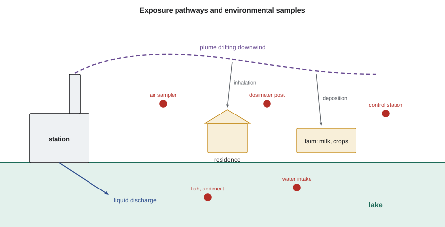
A good program samples each important exposure pathway at the places where people would receive the highest dose, and at control locations far enough away to be unaffected. The critical group, or representative person, is the group expected to receive the highest dose, for example a farm family downwind who drink their own milk and eat their own vegetables. Sampling locations are chosen using the site's meteorology, the prevailing wind directions, the location of farms and water intakes, and land-use surveys repeated every few years.
Typical samples include continuous air samples drawn through particulate filters and charcoal cartridges, changed weekly; tritium in air collected by water vapor samplers; direct radiation measured by passive dosimeters on posts around the site; drinking water and surface water; groundwater from monitoring wells; milk, crops and garden produce; fish and sediments. Each sample type has a set frequency and set analyzes.
| Sample | Typical frequency | Main analyzes |
|---|---|---|
| Air particulate filter | Weekly | Gross beta; gamma spectroscopy of composites |
| Air charcoal cartridge | Weekly | Radioiodine by gamma spectroscopy |
| Air water vapor | Weekly or monthly | Tritium by liquid scintillation |
| Direct radiation dosimeters | Quarterly | Ambient dose equivalent |
| Drinking and surface water | Weekly to monthly | Tritium, gamma spectroscopy, gross beta |
| Groundwater wells | Quarterly | Tritium, gamma spectroscopy |
| Milk | Monthly or more often in grazing season | Iodine-131, cesium-137, strontium-90 |
| Fish and sediment | Twice a year | Gamma spectroscopy |
Measuring very low activities
Environmental samples contain activities thousands of times lower than the samples Hana counted in earlier lessons, often comparable to natural background. Everything in lesson 1 about detection limits matters here. Laboratories use large sample volumes, chemical concentration, long counting times and low-background detectors to reach detection limits low enough to be useful. Required lower limits of detection are set in licenses or monitoring standards for each sample type and radionuclide.
# Environmental monitoring: decay correction, MDA of a water sample and a dose estimate.
import math
half = {'H-3': 12.32 * 365.25, 'Cs-137': 30.08 * 365.25, 'I-131': 8.02, 'Co-60': 5.27 * 365.25}  # days
def decay_back(A_meas, nuc, days):
    return A_meas * math.exp(math.log(2) / half[nuc] * days)
print(f"I-131 measured 0.40 Bq/L, 6 days after collection -> {decay_back(0.40, 'I-131', 6):.2f} Bq/L at collection")

# MDA (Currie) for a gamma count of a 1 L water sample
B, t, eff, y, V = 900, 60000.0, 0.03, 0.851, 1.0
LD = 2.71 + 4.65 * math.sqrt(B)
MDA = LD / (eff * y * t * V)
print(f"Cs-137 MDA: {MDA*1000:.1f} mBq/L")

# Tritium in drinking water: dose from a year at a measured concentration
conc = 12.0            # Bq/L (illustrative)
intake = 730           # L per year
dcf = 1.8e-11          # Sv per Bq ingested, tritiated water (approx.)
print(f"annual dose: {conc*intake*dcf*1e6:.3f} microsievert")I-131 measured 0.40 Bq/L, 6 days after collection -> 0.67 Bq/L at collection Cs-137 MDA: 92.8 mBq/L annual dose: 0.158 microsievert
The program shows a one-liter water sample counted for about 17 hours on a germanium detector, giving a cesium-137 MDA of about 0.09 Bq/L. Reaching lower values needs larger samples, evaporation or ion exchange to concentrate the activity, or a more efficient detector. Short-lived radionuclides such as iodine-131 must also be decay-corrected to the time of collection, since a week or more can pass between collection and counting. The correction is
Six days of delay raise an iodine-131 result by two thirds; for cesium-137 the same delay is negligible. Composite samples, such as a month of weekly air filters counted together, need decay correction for each part from its own collection time, or a correction based on the midpoint of collection when the half-life is long compared with the compositing period.
Background and the meaning of a positive result
Environmental samples always contain natural radioactivity: potassium-40 in milk and fish, radon progeny on air filters, beryllium-7 produced by cosmic rays and deposited from the atmosphere, uranium and thorium decay products in soil and sediment, and cesium-137 from atmospheric weapons testing in the 1950s and 1960s and from the 1986 Chernobyl and 2011 Fukushima accidents. Tritium and carbon-14 are produced naturally in the atmosphere as well. A positive result for a radionuclide that a station also releases does not by itself show that the station caused it.
Distinguishing station contributions relies on several lines of evidence. Indicator locations near the station should show higher values than control locations in the same period. The ratio of radionuclides should match the station's releases rather than global fallout. Results should correlate with wind direction and with release records. And results should be compared with the long-term record at the same location, which is why programs keep decades of data. Hana learns that most positive results at control locations are fallout cesium in soil and sediments, and most at indicator locations are tritium, which CANDU stations release in larger amounts than light water reactors.
For a US light water reactor, tritium in groundwater monitoring wells has received particular attention since leaks from buried piping were found at several plants in the 2000s, leading to an industry groundwater protection initiative. The EPA drinking water standard for tritium is 20 000 pCi/L, about 740 Bq/L, and results near the plants are typically far below that value.
From concentrations to dose
Environmental results are turned into dose estimates by multiplying a measured concentration by an intake rate and a dose coefficient. For drinking water, the annual dose is
where \(C\) is the concentration in becquerels per liter, \(I\) the annual water intake and \(e_{\text{ing}}\) the ingestion dose coefficient in sieverts per becquerel. The program uses a tritium concentration of 12 Bq/L, 730 liters per year and a tritiated water coefficient of about \(1.8 \times 10^{-11}\) Sv/Bq, giving about 0.16 µSv per year, roughly one ten-thousandth of the dose most people receive each year from natural background. Similar calculations, done in the station's dose models for all pathways, give the annual public dose reported to the regulator.
Direct radiation from the station is measured by dosimeters placed on posts at the site boundary and beyond, with control dosimeters far away. Because natural background varies with soil, building materials and season, small differences between locations are expected. The program compares each location with its own long-term average and with controls exposed at the same time, and investigates statistically significant changes.
Quality assurance for environmental data
Environmental data are often seen by the public, by local communities and Indigenous nations, and by regulators, and they must be defensible. Laboratories participate in interlaboratory comparison programs in which they analyze samples of known activity prepared by a reference laboratory. They analyze blind duplicates and spiked samples, track their own control charts and document every result from collection to report. Chain-of-custody forms follow each sample. The next lesson develops these quality assurance tools in detail.
Environmental programs also respond to events. After an unplanned release, sampling frequency increases, additional locations are added, and samples are analyzed faster. Emergency preparedness, the subject of a lesson in NUC-320, relies on the same equipment and staff, so practicing routine environmental work well also maintains the capacity for emergencies.
Continuous effluent monitors
At the stack and in liquid discharge lines, continuous monitors provide real-time indication of releases and can trigger alarms or automatic isolation if a limit is approached. Stack monitors draw a representative air sample through a particulate filter, which is viewed by a beta or gamma detector, then through a charcoal or silver zeolite cartridge for radioiodine, and finally past a shielded noble gas chamber. Tritium is sampled separately by collecting water vapor or by ionization chambers that subtract the gamma background. Liquid monitors use NaI or plastic detectors on a sample line or in a shielded well around the discharge pipe.
Continuous monitors are not as sensitive as laboratory analysis, so their role is to show trends and give early indication of problems, while the release totals used for dose calculations come from composite samples analyzed in the laboratory. The monitors' alarm setpoints are calculated from the derived release limits or dose objectives, with margins for uncertainty, and are documented in the station's effluent program. Isokinetic sampling, matching the sampler's intake velocity to the stack flow, is needed to collect particles representatively; a sampler drawing too fast or too slow collects too few or too many large particles.
Communicating results
Environmental data matter to people who live near a station, and reports are written for them as well as for specialists. Good practice presents results in context: comparing them with natural background, with drinking water standards and with the doses people receive from everyday sources such as air travel or medical imaging. Numbers below detection limits are reported as such, not as zero. Trends over many years are shown in graphs, and any result above normal levels is explained, including when the explanation is a laboratory error. Openness about small problems is what builds the credibility needed if a real event ever occurs.
Many stations involve local communities and Indigenous nations in their monitoring programs, through community sampling of traditional foods, joint sampling events or independent review of results. These arrangements recognize that people value being able to see and test the data themselves, and they often improve the program by identifying pathways and foods that the original design missed.
Sample collection and handling
Most errors in environmental results arise before a sample reaches a detector. Air samplers must run at their calibrated flow rate for the whole period, and a power failure or a clogged filter that reduces the volume sampled must be recorded so that the concentration is calculated correctly. Water samples are acidified to keep dissolved radionuclides from sticking to container walls. Milk is kept cold and analyzed quickly for iodine-131. Vegetation and fish samples are weighed fresh and again after drying or ashing, so results can be reported in the basis the program requires. Each sample is labeled with location, date, time, collector and sample volume or mass, and its chain-of-custody form records every person who handled it. A missing or ambiguous label can make an otherwise good result useless.
Field blanks, containers filled with clean water and carried through the same handling as real samples, reveal contamination introduced in the field or the laboratory. Duplicate samples collected side by side show the combined variability of sampling and analysis, which is often larger than the counting uncertainty alone.
Hana's field day
Hana's sampling round ends at the control station, a farm thirty kilometers upwind. Its air filter shows radon progeny and beryllium-7 but nothing else; the indicator station's filter, closest to the station, looks the same. The tritium in water vapor at the indicator station is measurable but low, and consistent with the stack release record for the week. She writes up the round in the format the annual report uses, and notes for Marcel that every number in it depends on the counting statistics of lesson 1, the detectors of lessons 3 and 4, and the calibrations of lesson 11.
Summary and key terms
- Effluent monitoring measures releases; environmental monitoring confirms doses and detects unexpected pathways.
- Programs sample each pathway at critical-group locations and at upwind or distant controls.
- Low activities need large samples, concentration, long counts and low-background detectors.
- Short-lived results are decay-corrected to collection: A₀ = A exp(λt).
- Natural radioactivity and global fallout must be separated from station contributions.
- Dose = concentration × intake × dose coefficient; public doses are small fractions of natural background.
- Effluent monitoring
- Measurement of radioactivity released from a facility to air and water.
- Exposure pathway
- A route by which radioactivity reaches people, such as inhalation or milk.
- Representative person
- A hypothetical individual receiving a dose typical of the most exposed group.
- Indicator location
- A sampling point where station effects would be greatest.
- Control location
- A sampling point far enough away to be unaffected by the station.
- Composite sample
- Several samples combined for a single analysis.
- Dose coefficient
- The committed dose per unit intake of a radionuclide.
Practice problems
Work each problem on paper first, then reveal the answer to check.
An I-131 result of 0.2 Bq/L is measured 8 days after collection. Value at collection?
Show answer
About 0.4 Bq/L (one half-life).
Why are control locations needed?
Show answer
To show what background and fallout look like without the station's influence.
Using 730 L/yr and 1.8 × 10⁻¹¹ Sv/Bq, what dose does 100 Bq/L of tritium give?
Show answer
100 × 730 × 1.8 × 10⁻¹¹ ≈ 1.3 µSv per year.
Why is beryllium-7 found on air filters everywhere?
Show answer
It is produced by cosmic rays in the atmosphere and deposited naturally.
How can an analyst tell fallout cesium from station cesium?
Show answer
By location patterns, radionuclide ratios, correlation with releases and the long-term record.
Name two ways to lower the MDA of a water sample.
Show answer
Larger volume or concentration, longer count, more efficient or lower-background detector.
Lesson quiz · 5 questions
Score 60% or more to complete this lesson.
Create a free account to save your progress, take quizzes and earn a certificate.