Laboratory practice

The last lesson of the course is practical. Before Hana's secondment ends, Marcel asks her to run the training laboratory that new technicians complete before they are authorized to work in the counting room, and to write it up so that it can be used with the next group. The experiments use sealed check sources and the a university TRIGA research reactor for activation samples, and each one ties back to a lesson in this course. This lesson describes those experiments, the safe working practices that surround them, and what each teaches.

Working safely with sources

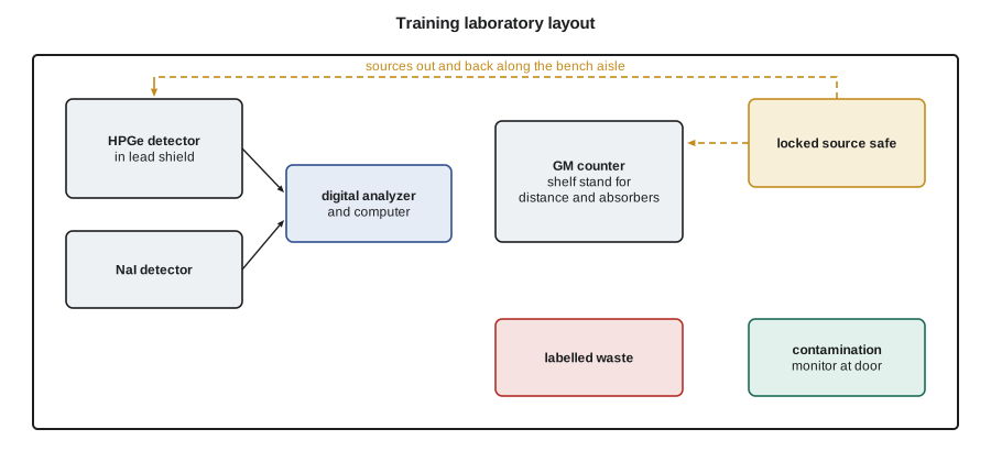
Every experiment in the laboratory uses sealed sources or small activated samples, and the rules are the same as in any radiation laboratory. Sources are signed out from a locked store and signed back in at the end of the session. Students wear a dosimeter and use a contamination monitor at the exit. Sources are handled with tongs or by their holders, never directly, and kept shielded when not in use. The three principles of time, distance and shielding, developed in NUC-320, apply even to small sources: spending less time close to a source, standing back, and working behind shielding all reduce dose.

Sealed sources are leak-tested at regular intervals by wiping them and counting the wipe, a direct use of the low-level counting methods of lesson 1. Activated foils and samples from the research reactor are unsealed and must be handled in trays with absorbent liners and monitored for contamination. Any spill is reported immediately. Eating, drinking and applying cosmetics are forbidden in the laboratory, and hands are monitored on leaving.

The laboratory's sources are held under an NRC or Agreement State radioactive materials license, which sets conditions for storage, inventory, leak testing and the training of users, and the activation work at the TRIGA follows the research reactor's own license and procedures.

Experiment 1: The GM plateau and counting statistics

The first experiment characterizes a Geiger-Mueller counter. With a beta check source in a fixed position, students record the count rate as they raise the high voltage in steps. Below the starting voltage no counts appear; above it the rate rises quickly to a plateau and then rises again as continuous discharge begins. The operating voltage is chosen about a third of the way along the plateau, and the plateau slope is expressed in percent per 100 V. A healthy halogen-quenched tube has a slope of a few percent per 100 V or less.

# Laboratory practice: two-source dead time, a counting plateau and inverse square check.
import math
r1, r2, r12, rb = 2850.0, 3120.0, 5620.0, 2.0       # cps
tau = (r1 + r2 - r12 - rb) / (r12**2 - r1**2 - r2**2)
print(f"two-source dead time estimate: {tau*1e6:.0f} microseconds")

# GM plateau: counts vs voltage, find slope in % per 100 V
plateau = [(900, 0), (950, 3820), (1000, 4010), (1100, 4065), (1200, 4120), (1300, 4190), (1400, 5300)]
v1, c1 = plateau[2]; v2, c2 = plateau[5]
slope = (c2 - c1) / c1 * 100 / ((v2 - v1) / 100)
print(f"plateau slope {slope:.2f} % per 100 V; operate near {(v1+v2)/2:.0f} V")

# Inverse square check with a sealed source
for d in (10, 20, 40):
    print(f"distance {d:3d} cm: expected relative rate {(10/d)**2:6.4f}")

two-source dead time estimate: 25 microseconds
plateau slope 1.50 % per 100 V; operate near 1150 V
distance  10 cm: expected relative rate 1.0000
distance  20 cm: expected relative rate 0.2500
distance  40 cm: expected relative rate 0.0625

With the voltage set, students make twenty one-minute counts of the same source and compare their scatter with Poisson statistics using the chi-square test from lesson 11. They also count background for the same time and calculate the net rate and its uncertainty as in lesson 1. Most students are surprised by how much the counts vary, and the experiment is designed to make the square-root rule something they have seen rather than only read about.

Experiment 2: Dead time by the two-source method

The dead time of a counting system can be measured with two sources of similar activity, each giving a high count rate. Students count source 1 alone, both sources together, source 2 alone and background, with the sources returned to exactly the same positions each time. Because the combined rate is high, more counts are lost to dead time when both sources are present, and the sum of the individual rates exceeds the combined rate. For a non-paralyzable system, the dead time is approximately

The program applies this to one set of results and finds about 25 µs. The method is sensitive to small errors in source position, since the result depends on a small difference between large rates, and students repeat it to see how much the estimate varies. The lesson is a practical one: measure dead time, but do not trust a single measurement, and always keep count rates low enough that dead-time corrections are small.

Experiment 3: The inverse square law and attenuation

A small gamma source is placed at a series of distances from a detector, and the net count rate is compared with the inverse square law. Close to the source, the detector's finite size and the position of the effective point of interaction within it cause deviations, and students fit an effective distance offset. They then place absorbers of increasing thickness between the source and detector and plot the logarithm of the count rate against thickness to find the linear attenuation coefficient and half-value layer. The difference between narrow-beam and broad-beam geometry, where scattered photons reach the detector, introduces the buildup factor treated in NUC-320.

Experiment 4: Gamma spectroscopy with NaI and germanium

Students record spectra of cesium-137, cobalt-60 and a mixed source with a NaI detector and then with an HPGe detector. They perform an energy calibration, measure the FWHM of each peak and compare the two detectors' resolution with the values predicted in lessons 3 and 4. They identify the photopeaks, Compton edges, backscatter peaks and lead X-rays, and calculate the Compton edge energies from lesson 5 to check their assignments.

Then they receive an unknown sample, a sealed mixture whose contents are known only to the instructor. They must identify every radionuclide, calculate its activity using the laboratory's efficiency calibration and report it with an uncertainty. Their results are scored like a proficiency test. Hana's first group of trainees identifies all four radionuclides, but two of them miss a weak line hidden on a Compton edge, the same mistake she made with the resin sample in lesson 5.

Experiment 5: Neutron activation and half-life

Thin foils of indium, gold or copper are irradiated for a known time in the research reactor and counted afterwards. The activity at the end of irradiation depends on the flux, the activation cross section and the number of target atoms, and approaches saturation for long irradiations:

Students count the indium-116m activity repeatedly as it decays, plot the logarithm of the count rate against time and find the half-life, about 54 minutes. They then work backward from the measured activity to estimate the thermal neutron flux at the irradiation position, and compare it with the facility's published value. Covering one foil with cadmium, which absorbs thermal neutrons, gives the cadmium ratio introduced in NUC-300 and shows how much of the activation comes from epithermal neutrons.

A TRIGA research reactor provides a range of irradiation positions, and many universities use them for exactly this kind of teaching experiment as well as for neutron activation analysis.

Experiment 6: Liquid scintillation and quench

Students prepare a set of vials containing the same tritium activity but different amounts of a quenching agent, count them on a liquid scintillation counter and plot efficiency against the instrument's quench indicator. They then count an unknown water sample and use the quench curve to determine its tritium concentration. The experiment shows why every sample needs a quench correction and how much results would be biased if a single efficiency were used.

Experiment 7: Dosimeters

Pairs of TLD chips and an electronic dosimeter are placed at measured distances from a calibrated cesium-137 source for a set time. Students calculate the expected dose from the source's air kerma rate constant and the inverse square law, then read the TLDs and EPD and compare. Differences of 10 to 20 % are common and are traced to energy response, positioning and the uncertainty of the reference calculation. The exercise links the dosimetry of lesson 8 with the calibration ideas of lesson 11.

Laboratory records and reports

Each experiment is written up in a standard format: purpose, equipment with serial numbers and calibration dates, settings, raw data, calculations with uncertainties, results compared with expectations, and a short discussion of discrepancies. Raw data are recorded in ink or saved electronically without editing; corrections are made by striking through and initialling. That format is the same one the counting room uses for its working records, so trainees learn it before their results start to matter.

Marcel's grading emphasizes the discussion. A result that disagrees with expectation by more than its uncertainty is not a failure if the student explains it correctly and identifies what would fix it. A result that agrees perfectly but has no uncertainty, or uses the wrong time, loses marks. Good measurement practice is as much about honest reporting as about getting the expected number.

Professional responsibility

The final page of Hana's write-up is about responsibility. Radiation measurements protect workers, the public and the environment, and they underpin the trust that communities place in nuclear facilities. Every number reported carries the name of the person who measured it and the person who reviewed it. If a result is surprising, it is checked, not adjusted. If a measurement cannot be made with the required quality, that is reported. And if a practice is unsafe, anyone in the laboratory can stop it. Professional engineers and technologists have codes of ethics that say the same thing in more formal words.

Dr. Vasquez reads the write-up when Hana returns to the core physics group. Her only comment is that the reactor physicists use every detector in this course, from the source-range counters that watch the approach to critical to the in-core detectors that check the physics model. Understanding how those measurements are made, and how they can go wrong, will make Hana a better physicist.

Common errors in the training laboratory

Marcel keeps a list of the errors trainees make most often, because each one also appears in real work. Background is measured once at the start of the session and never again, even though the room's background changes when other groups bring out sources. Counting time is taken from a wall clock rather than the instrument's timer. Sources are placed at slightly different positions in repeat counts, which adds variation that students then blame on statistics. Units are mixed, such as counts per minute in one column and counts per second in another. Decay correction is forgotten for short-lived activation products. And uncertainties are calculated from rates instead of counts. Each item on the list is now a check box on the laboratory report form, and Hana's first group makes fewer of them than the last.

Marcel also asks each trainee to explain one result to a non-specialist, in plain words, at the end of the course. Being able to say what a number means, and how sure we are of it, is part of the job.

At the end of every session, the instructor and trainees complete a short close-out: all sources returned and the store log signed, a contamination survey of benches and hands recorded, waste segregated into labeled containers, and instruments switched off or left in their monitoring state. The close-out takes ten minutes, and it is the habit that keeps a laboratory clean and its inventory accurate over years of use.