
GEOM-440 · Lesson 8 of 12 · 20 min
Deep learning for imagery
The district's field boundaries were digitized years ago from air photos and have been patched ever since. Fields have been split, joined and re-shaped by pivots, and the GIS lags behind. Each spring a ditch rider marks changes on paper maps, and Theo enters them weeks later. Marta asked whether the imagery could find the changes automatically. Drawing boundaries is something people do by seeing edges, shapes and textures together, and it is exactly the kind of task where deep learning has transformed image analysis. This lesson explains how convolutional networks work, how they are trained and tested for geospatial tasks, and what the district's boundary project needed to make them useful.
From pixels to learned features
The classifiers of lesson 7 work on features a person chose: band values, indices, textures. A convolutional neural network, CNN, learns its own features from the pixels. Its basic operation is convolution: a small grid of weights, the kernel, slides over the image and at each position computes a weighted sum of the pixels beneath it. A kernel with positive weights on one side and negative on the other responds to edges; others respond to spots, lines or textures. The first layer of a trained network typically contains such edge and color detectors, learned rather than designed.
Each layer applies many kernels, producing a stack of feature maps, and passes them through a nonlinearity, usually the rectified linear unit, ReLU, which sets negative values to zero. Pooling layers shrink the maps, typically halving their size by keeping the maximum of each two-by-two block. Stacking convolutions and pooling builds features of growing size and abstraction: edges, then corners and textures, then field patterns, center-pivot circles, farmyards. The receptive field of a unit, the patch of input it can see, grows with depth, which lets deep layers recognise large structures.
Network designs for geospatial tasks
| Task | Output | Typical architecture |
|---|---|---|
| Scene classification | One label per image tile | ResNet-style CNN or vision transformer |
| Semantic segmentation | A label for every pixel | U-Net, DeepLab |
| Object detection | Boxes around objects, such as farm buildings or bales | Faster R-CNN, YOLO family |
| Instance segmentation | A separate mask for each object, such as each field | Mask R-CNN, or segmentation plus post-processing |
| Change detection | Changed pixels between two dates | Siamese networks over two images |
| Time series classification | A label from a sequence of images | Temporal CNNs, recurrent networks, transformers |
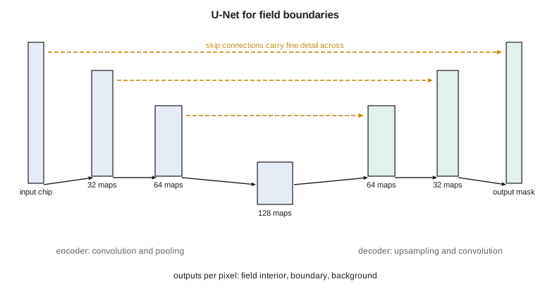
Field boundary mapping is a segmentation problem. The U-Net, designed for medical images in 2015 and now standard in remote sensing, has an encoder that convolves and pools the image down to coarse, rich features, and a decoder that upsamples them back to full resolution. Skip connections pass the encoder's fine-detail maps across to the decoder at each scale, so the output has both context and sharp edges. For fields, a common design predicts three outputs per pixel: the field interior, the boundary, and the distance to the nearest boundary. Combining them with a watershed step separates touching fields into individual polygons.
Training
Training adjusts millions of weights to minimize a loss function on labeled examples, by gradient descent: compute the loss on a batch of image chips, compute how the loss changes with each weight by backpropagation, and move every weight a small step downhill. For segmentation, the loss compares predicted and reference masks pixel by pixel, with cross-entropy or with losses based on overlap, such as Dice, that cope better when one class, such as boundary pixels, is rare.
Labels are the bottleneck. The district's 1,100 fields give perhaps 10,000 chips of 256 by 256 pixels at 10 m, and each needs a reference mask. Theo's team drew masks from the existing GIS, after correcting the 80 fields known to be out of date, and checked a sample against new air photos. Data augmentation multiplies the examples by flipping, rotating and shifting the chips, and by small changes of brightness, since a field rotated 90° is still a field. Transfer learning starts from a network pretrained on a large dataset and fine-tunes it on the local data, which needs far fewer labels than training from scratch.
Since about 2023, geospatial foundation models have been released: large networks pretrained by self-supervision on huge archives of satellite imagery, such as the Prithvi models from NASA and IBM, built on harmonized Landsat and Sentinel-2 data. Fine-tuned on a few hundred labeled examples, they can match networks trained from scratch on many thousands, especially for tasks that use time series. Their value for a small district is that the expensive learning has already been done elsewhere. Their risk is that their behavior on local conditions, such as narrow irrigated strips in dry prairie, must still be tested locally.
Testing a segmentation model
Pixel accuracy is a poor measure for segmentation: a model that labels every pixel as field interior scores well, because boundaries are few. Intersection over union, IoU, compares the predicted and reference sets for a class as the area of their overlap divided by the area of their union. For boundaries, a tolerance matters: a predicted boundary one pixel off is usually acceptable, so boundary precision and recall are computed by matching boundary pixels within a buffer. For field objects, the practical test counts how many reference fields are matched by one predicted field with high IoU, how many are over-segmented into pieces and how many are merged with neighbors.
The warnings of lesson 7 apply with extra force. Chips cut from one image overlap, and neighboring chips share fields, so random splits of chips into training and test sets leak. The firm's split holds out whole townships, about 10 km squares, and one whole year of imagery, so that the test measures both spatial and temporal generalization.
The code below shows the core operations at a scale small enough to follow: a 3 by 3 edge-detecting kernel convolved over a small image of two fields and a road, ReLU and max pooling, the receptive field of a U-Net encoder, and IoU and boundary precision and recall for a predicted mask.
# A 10 x 10 vegetation index image: two fields separated by a road (column 5)
img = [[0.75 if c < 5 else (0.20 if c == 5 else 0.45) for c in range(10)] for r in range(10)]
k = [[-1, 0, 1], [-2, 0, 2], [-1, 0, 1]]            # Sobel kernel: responds to vertical edges
def conv(x, k):
    n = len(x); m = len(x[0])
    return [[sum(k[u][v] * x[r + u - 1][c + v - 1] for u in range(3) for v in range(3))
             for c in range(1, m - 1)] for r in range(1, n - 1)]
y = [[max(0.0, abs(v)) for v in row] for row in conv(img, k)]         # |response| then ReLU
print("edge response along one row:", [round(v, 2) for v in y[3]])
pool = [[max(y[r][c], y[r][c + 1], y[r + 1][c], y[r + 1][c + 1]) for c in range(0, 8, 2)] for r in range(0, 8, 2)]
print("after 2x2 max pooling     :", [round(v, 2) for v in pool[1]])

# receptive field of an encoder: two 3x3 convolutions then a 2x2 pool, four times
rf, jump = 1, 1
for level in range(1, 5):
    for _ in range(2): rf += 2 * jump
    rf += jump; jump *= 2
    print(f"level {level}: receptive field {rf:3d} px = {rf * 10:5d} m at 10 m pixels")

# IoU and boundary precision/recall (tolerance 1 px) for a predicted field mask
ref = {(r, c) for r in range(2, 9) for c in range(2, 8)}
pred = {(r, c) for r in range(2, 9) for c in range(2, 9) if not (r == 8 and c == 8)}
iou = len(ref & pred) / len(ref | pred)
def edge(S): return {p for p in S if any((p[0] + a, p[1] + b) not in S for a, b in ((1, 0), (-1, 0), (0, 1), (0, -1)))}
er, ep = edge(ref), edge(pred)
near = lambda p, E: any(abs(p[0] - q[0]) <= 1 and abs(p[1] - q[1]) <= 1 for q in E)
prec = sum(near(p, er) for p in ep) / len(ep); rec = sum(near(p, ep) for p in er) / len(er)
print(f"IoU {iou:.3f}; boundary precision {prec:.2f}, recall {rec:.2f}, F1 {2 * prec * rec / (prec + rec):.2f}")edge response along one row: [0.0, 0.0, 0.0, 2.2, 1.2, 1.0, 0.0, 0.0] after 2x2 max pooling : [0.0, 2.2, 1.2, 0.0] level 1: receptive field 6 px = 60 m at 10 m pixels level 2: receptive field 16 px = 160 m at 10 m pixels level 3: receptive field 36 px = 360 m at 10 m pixels level 4: receptive field 76 px = 760 m at 10 m pixels IoU 0.875; boundary precision 1.00, recall 1.00, F1 1.00
The kernel responds strongly on both sides of the road and not at all inside the fields, and pooling keeps the strong responses while halving the resolution. The receptive field grows quickly with depth: after four levels a unit sees 76 pixels, 760 m at 10 m, about the width of a quarter section, which is why deep layers can use context such as the shape of a pivot circle. The predicted mask is one column too wide, so IoU is 0.875, yet boundary precision and recall within a one-pixel tolerance are both perfect: the error is a shift of one edge by a single pixel, which a boundary score with tolerance forgives entirely and IoU does not. Which measure to report depends on the use. For updating the GIS, a one-pixel shift at 10 m is within the accuracy of the old digitizing, so the boundary score is the more relevant one; for estimating field areas, IoU is.
import torch, torch.nn as nn

def block(i, o):
    return nn.Sequential(nn.Conv2d(i, o, 3, padding=1), nn.BatchNorm2d(o), nn.ReLU(inplace=True),
                         nn.Conv2d(o, o, 3, padding=1), nn.BatchNorm2d(o), nn.ReLU(inplace=True))
class UNet(nn.Module):
    def __init__(self, bands=12, classes=3, w=32):
        super().__init__()
        self.e1, self.e2, self.e3 = block(bands, w), block(w, 2 * w), block(2 * w, 4 * w)
        self.pool = nn.MaxPool2d(2)
        self.u2 = nn.ConvTranspose2d(4 * w, 2 * w, 2, stride=2); self.d2 = block(4 * w, 2 * w)
        self.u1 = nn.ConvTranspose2d(2 * w, w, 2, stride=2); self.d1 = block(2 * w, w)
        self.out = nn.Conv2d(w, classes, 1)          # interior, boundary, background
    def forward(self, x):
        a = self.e1(x); b = self.e2(self.pool(a)); c = self.e3(self.pool(b))
        d = self.d2(torch.cat([self.u2(c), b], 1))    # skip connection
        e = self.d1(torch.cat([self.u1(d), a], 1))    # skip connection
        return self.out(e)
model = UNet()
opt = torch.optim.AdamW(model.parameters(), lr=1e-3)
loss_fn = nn.CrossEntropyLoss(weight=torch.tensor([1.0, 5.0, 1.0]))   # boundaries are rare
Running a trained model over the district is called inference. Images are cut into overlapping tiles, predicted tile by tile, and stitched back together, keeping only the central part of each tile's prediction, because predictions near tile edges lack context and are less reliable. A graphics processor makes both training and inference practical: training the district's model took a few hours on one rented cloud GPU, and inference over the whole district takes minutes. The cost of the computing is small next to the cost of the labels and the checking.
Worked problem
Intersection over union
A reference field covers 420 pixels. The predicted field covers 450 pixels, of which 400 overlap the reference. Compute IoU and the Dice coefficient.
Show solution
- \[\text{union} = 420 + 450 - 400 = 470\]
- \[\text{IoU} = 400/470 = 0.851\]
- \[\text{Dice} = \frac{2 \times 400}{420 + 450} = 0.920\]
Answer: IoU ≈ 0.85 and Dice ≈ 0.92; Dice is always the larger of the two for imperfect overlap.
Coulee Geomatics: the boundary update
The boundary model the firm deployed starts from a pretrained foundation model, fine-tuned on the district's corrected masks and tested on two held-out townships and the 2025 season. It matches 91 percent of reference fields with IoU above 0.8. More useful to Marta than the score is the workflow it supports: each spring the model runs on the new imagery, the fields whose predicted outline differs from the GIS by more than a set area are flagged, and Theo reviews the flagged list, usually a few dozen fields, instead of the whole district. Nothing changes in the GIS without a person accepting it.
Common mistakes
MistakeJudging a segmentation model by pixel accuracy.
InsteadUse IoU, Dice and boundary scores with a tolerance, and object matching counts.
MistakeSplitting overlapping chips randomly between training and test.
InsteadHold out whole areas and whole years.
MistakeTraining a large network from scratch on a few hundred labels.
InsteadUse transfer learning or a pretrained foundation model, with augmentation.
MistakeWriting model outputs straight into the authoritative GIS.
InsteadUse predictions to flag changes for review by a person.
Summary and key terms
- CNNs learn features by convolving kernels over images, with nonlinearities and pooling.
- Receptive fields grow with depth, letting deep layers use context.
- U-Nets combine an encoder, a decoder and skip connections for pixel-level segmentation.
- Training uses gradient descent on labeled chips; labels and augmentation are the bottleneck.
- Foundation models pretrained on large image archives reduce the labels needed locally.
- Evaluate with IoU, boundary scores and spatially and temporally held-out tests.
- Convolution
- Sliding a kernel of weights over an image and summing products at each position.
- ReLU
- The rectified linear unit, max(0, t).
- Receptive field
- The patch of input that affects one unit of a layer.
- U-Net
- An encoder-decoder segmentation network with skip connections.
- Transfer learning
- Starting from a network trained on another dataset and fine-tuning it.
- IoU
- Intersection over union of predicted and reference regions.
Practice problems
Work each problem on paper first, then reveal the answer to check.
What does max pooling with a 2 by 2 window do to a feature map?
Show answer
It halves each dimension, keeping the largest value in each block.
Why are skip connections used in a U-Net?
Show answer
To pass fine spatial detail from the encoder to the decoder.
Why is cross-entropy weighted toward the boundary class?
Show answer
Boundary pixels are rare, so unweighted training would neglect them.
A model labels every pixel as interior. Why can its pixel accuracy still be high?
Show answer
Most pixels are interior; pixel accuracy hides the failure on rare classes.
What does a geospatial foundation model offer a small project?
Show answer
Pretrained features that need far fewer local labels to fine-tune.
Lesson quiz · 5 questions
Score 60% or more to complete this lesson.
Create a free account to save your progress, take quizzes and earn a certificate.