
GEOM-440 · Lesson 7 of 12 · 21 min
Machine learning on spatial data
The crop map from the remote sensing program in GEOM-320 was built with a classifier trained on about 300 field visits a season. It reported an overall accuracy of 94 percent, and for two seasons nobody questioned it. Then Leah, rebuilding the classifier for the analytics program, repeated the accuracy test in a different way and got 81 percent. Nothing about the map had changed. What changed was how the test data were chosen. This lesson is about machine learning on spatial data, and its central warning: models learn from neighbors, and tests that let them see their test data's neighbors report accuracy they do not have.
Learning from examples
Supervised machine learning fits a function from features to a target using labeled examples. For the crop map, each pixel's features are its reflectances and vegetation indices on several image dates, and the target is its crop. For a regression task, such as predicting soil salinity from remote sensing and terrain, the target is a number. The learner chooses the function from a family, such as all decision trees of a given depth, by minimizing error on the training examples, with some form of regularization to avoid memorizing them.
| Method | How it works | Strengths and cautions |
|---|---|---|
| k nearest neighbors | Predicts from the k most similar training examples in feature space | Simple, no training; slow on large data, sensitive to feature scaling |
| Random forest | Averages many decision trees, each grown on a bootstrap sample with random subsets of features | Robust default for tabular and pixel data; feature importances can mislead |
| Gradient boosting | Adds small trees one at a time, each fitting the errors of the ensemble so far | Often most accurate on tables; needs tuning and early stopping |
| Support vector machine | Finds a maximum-margin boundary, possibly in a transformed space | Good with few examples; less used now for large data |
| Neural networks | Layers of weighted sums and nonlinearities trained by gradient descent | Excel with images and sequences; need much data, lesson 8 |
Random forests became the workhorse of land cover mapping because they handle many correlated features, need little tuning and rarely overfit badly. Each tree splits the data on thresholds of single features; the forest's vote smooths out the quirks of any one tree. The out-of-bag error, computed on the samples each tree did not see, is a convenient built-in accuracy estimate, but for spatial data it inherits the problem this lesson is about: the samples left out of a tree are mostly neighbors of samples it did see.
Features that carry space
Spatial machine learning gains much from features engineered with geography in mind. Texture measures, summarizing the variation of values in a moving window, help separate crops with similar spectra but different row structure. Terrain features from the elevation model, such as slope, topographic wetness index and depth below the canal water level, help predict salinity. Distance to features, such as the canal or a lateral, encodes processes that act with distance. Coordinates themselves can be features, and sometimes improve accuracy, but they invite the model to memorize where things are rather than learn why, which fails as soon as it is applied elsewhere.
Object-based approaches classify segments rather than pixels: field polygons from the GIS, or segments grown from the image. Averaging pixels within a field removes noise and makes features such as field shape available. For the district, where field boundaries are known, classifying fields rather than pixels is both more accurate and closer to what the district needs: one crop per field.
Why random cross-validation lies
Cross-validation estimates how well a model will predict new data: split the labeled data into folds, train on all folds but one, test on the held-out fold, and repeat. With random folds, pixels from the same field end up in both training and test sets. Pixels in a field are nearly identical, so the test asks the model to recognise a field it has already seen. The estimate is then of interpolation within known fields, not of prediction for new fields, and it is too optimistic, sometimes by a wide margin. The same happens with any autocorrelated data: soil samples close together, or zones in the same reach.
Spatial cross-validation holds out whole groups: whole fields, spatial blocks larger than the range of autocorrelation, or buffers around each test point from which training data are excluded. The range from the variogram or correlogram of the target, or of the model's residuals, guides the block size. The resulting accuracy is lower and closer to what the map will achieve where it has no training data. Which estimate is right depends on how the model will be used. If the map's users only care about accuracy near the field visits, random folds are fair. If the map is used everywhere, as the crop map is, spatial folds are honest.
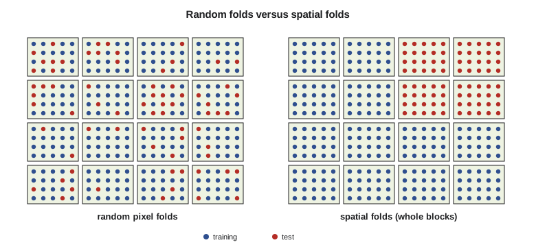
The code below builds a small version of the problem: 60 fields of three crops, 25 pixels each, with features on three image dates. Each field has its own offset from the crop's typical spectrum, from variety, seeding date and soil, and pixels within a field differ only slightly. A k-nearest-neighbor classifier is tested with five random folds of pixels and with five folds that keep whole fields together.
import math, random
random.seed(7)
crops = {"wheat": (0.35, 0.72, 0.40), "canola": (0.30, 0.65, 0.62), "barley": (0.33, 0.70, 0.48)}
pix = []                                         # (field, crop, features)
for f in range(60):
    crop = list(crops)[f % 3]
    off = [random.gauss(0, 0.05) for _ in range(3)]          # field effect: variety, timing, soil
    for _ in range(25):
        pix.append((f, crop, [m + o + random.gauss(0, 0.015) for m, o in zip(crops[crop], off)]))

def knn(train, x, k=5):
    near = sorted(train, key=lambda p: sum((a - b) ** 2 for a, b in zip(p[2], x)))[:k]
    votes = {}
    for p in near: votes[p[1]] = votes.get(p[1], 0) + 1
    return max(votes, key=votes.get)
def cv(fold_of):
    right = 0
    for k in range(5):
        train = [p for i, p in enumerate(pix) if fold_of(i, p) != k]
        test = [p for i, p in enumerate(pix) if fold_of(i, p) == k]
        right += sum(knn(train, p[2]) == p[1] for p in test)
    return right / len(pix)

order = list(range(len(pix))); random.shuffle(order); rf = {i: n % 5 for n, i in enumerate(order)}
fields = list(range(60)); random.shuffle(fields); ff = {f: n % 5 for n, f in enumerate(fields)}
a_rand = cv(lambda i, p: rf[i])
a_field = cv(lambda i, p: ff[p[0]])
print(f"pixels {len(pix)}, fields 60")
print(f"accuracy, random pixel folds : {a_rand:.3f}")
print(f"accuracy, whole-field folds  : {a_field:.3f}")
print(f"optimism from leakage : {a_rand - a_field:+.3f}")pixels 1500, fields 60 accuracy, random pixel folds : 0.926 accuracy, whole-field folds : 0.695 optimism from leakage : +0.231
With random folds of pixels, the classifier scores about 93 percent. With folds that keep whole fields together, it scores about 70 percent. The model has not changed; only the test has. With random folds, almost every test pixel has four or five pixels of its own field in the training set, and those neighbors carry the field's own offset from the typical spectrum, so the nearest neighbors vote correctly whether or not the classifier could recognise the crop in a field it had never seen. With whole-field folds, the classifier must generalize from other fields of the same crop, and the field-to-field variation, which is larger than the difference between wheat and barley on some dates, defeats it about three times in ten.
The gap of more than 20 percentage points is larger than in the district's real data, because the simulation makes the field effect large and the pixel noise small, but the direction is general. The more strongly the target and the features are autocorrelated, and the more the training data cluster, the larger the optimism of random folds. Five fields' worth of pixels are not five thousand independent examples; they are five examples, each seen many times.
import numpy as np, pandas as pd
from sklearn.ensemble import RandomForestClassifier
from sklearn.model_selection import GroupKFold, cross_val_score

px = pd.read_parquet("training_pixels_2026.parquet")        # features, crop, field_id, block_id
X = px.filter(like="b_").values; y = px.crop.values
rf = RandomForestClassifier(n_estimators=500, min_samples_leaf=2, n_jobs=-1, random_state=7)
random_cv = cross_val_score(rf, X, y, cv=5)                                   # optimistic
spatial_cv = cross_val_score(rf, X, y, cv=GroupKFold(5), groups=px.block_id)  # 2 km blocks
print(random_cv.mean(), spatial_cv.mean())
Leakage has other routes besides random folds. Tuning a model's settings, such as the number of neighbors or the depth of trees, on the same folds used to report accuracy makes the result optimistic again, because the settings were chosen to suit those folds; nested cross-validation, with an inner loop for tuning inside each outer spatial fold, avoids that. Features computed with a moving window can carry information from test pixels into training pixels if the window crosses a fold boundary, and scaling or imputing with statistics from the whole dataset leaks a little too. The rule is that everything learned from data, including preprocessing, must be learned from the training folds alone.
Accuracy that users can use
Overall accuracy hides much. A confusion matrix, met in GEOM-320, shows which classes are confused; user's and producer's accuracy say how reliable each class is from the map user's and the ground truth's points of view. For area estimation, the good-practice approach collects a probability sample of reference points after the map is made and uses it to estimate class areas with confidence intervals, correcting for the map's errors. Spatial cross-validation and a proper reference sample serve different purposes: the first guides model building, the second reports the map's accuracy to its users.
Uncertainty matters for machine learning predictions as for kriging. Random forests can give a class probability, the share of trees voting for each class, and quantile regression forests give prediction intervals for continuous targets. The area of applicability, a concept from the remote sensing literature, flags locations whose features are unlike any training data, where predictions should not be trusted at all. For the district, that flags the few organic soils near the reservoir, where no salinity samples exist.
Interpretation and fairness
Feature importance scores rank how much each feature helps a model, but with correlated features they can mislead: two bands that carry the same information split the credit, and dropping either changes little. Permutation importance, computed on spatially held-out data, is more reliable, and partial dependence plots show how predictions change with one feature. Explanations are not causes. A model that uses distance to the canal to predict salinity has learned an association; whether seepage causes it needs the kind of evidence the earlier lessons gathered.
Machine learning maps also shape decisions about people. If the salinity model is used to rank fields for drainage funding, errors fall on particular growers. Leah's team publishes the model's accuracy by area and by grower size, so that the board can see whether small holdings, with fewer samples, are predicted less well.
Worked problem
How much does leakage inflate accuracy?
A classifier scores 0.94 with random pixel folds and 0.81 with field-grouped folds on 1,500 pixels. The final map will be applied to 1,100 fields, of which 60 have training data. Which estimate better describes the map, and why?
Show solution
- \[\text{share of fields with training data} = 60/1100 \approx 0.055\]
- Random folds test pixels from fields the model has already seen, so they measure interpolation within visited fields.
- Grouped folds test fields the model has not seen, which is the situation for about 95 percent of the map.
Answer: The grouped estimate, about 0.81, describes the map far better; the random estimate applies only to the 5 percent of fields that were visited.
Coulee Geomatics: rebuilding the crop map
Leah's rebuilt classifier works on field objects, uses features from twelve image dates and texture from the 10 m bands, and is tested with folds of 2 km blocks, the distance at which the correlogram of the model's errors falls to zero. Its spatial cross-validated accuracy is 89 percent, better than the old map's honest 81 percent, and the area estimates now come with confidence intervals from a fresh random sample of 150 fields visited after the map was made. The 94 percent figure is retired from the district's reports, with a short note explaining why, which Marta forwards to the provincial agency that had been quoting it.
Common mistakes
MistakeTesting a spatial model with random folds of pixels or nearby samples.
InsteadHold out whole fields or spatial blocks larger than the autocorrelation range.
MistakeUsing coordinates as features without thinking about extrapolation.
InsteadPrefer process-related features; coordinates make models memorize places.
MistakeReporting random forest out-of-bag error as map accuracy.
InsteadOut-of-bag samples are neighbors of training samples; use spatial validation and a reference sample.
MistakeReading feature importance as causation.
InsteadUse permutation importance on held-out data and treat it as association.
Summary and key terms
- Supervised learning fits a function from features to targets using labeled examples.
- Random forests are a robust default for pixel and tabular geospatial data.
- Spatial features such as texture, terrain and distance often matter more than the learner.
- Random cross-validation of autocorrelated data leaks information and overstates accuracy.
- Spatial cross-validation holds out fields, blocks or buffered areas.
- Report map accuracy from a probability reference sample, and show where predictions apply.
- Supervised learning
- Fitting a model to examples with known targets.
- Random forest
- An ensemble of decision trees grown on bootstrap samples with random feature subsets.
- Cross-validation
- Estimating prediction error by repeatedly holding out part of the data.
- Data leakage
- Information from test data reaching the model during training or tuning.
- Spatial cross-validation
- Cross-validation with folds separated in space.
- Area of applicability
- The region of feature space, and hence of the map, where a model's training data support its predictions.
Practice problems
Work each problem on paper first, then reveal the answer to check.
Why do random folds overstate the accuracy of a crop classifier?
Show answer
Test pixels share fields with training pixels and are nearly identical to them.
How large should spatial blocks be?
Show answer
Larger than the range of autocorrelation of the target or of the model's errors.
Why can coordinates as features be risky?
Show answer
The model may memorize locations and fail where it has no training data.
What does a quantile regression forest add?
Show answer
Prediction intervals for a continuous target.
Why classify fields rather than pixels in the district?
Show answer
Field boundaries are known, averaging removes noise, and the district needs one crop per field.
Lesson quiz · 5 questions
Score 60% or more to complete this lesson.
Create a free account to save your progress, take quizzes and earn a certificate.