Spatial statistics

The first question the board asked was the simplest to state: are the canal seepage complaints clustered, or do they just look that way on a map? Over ten years, ditch riders and landowners logged wet spots, boggy field edges and white salt crusts near the canal and its laterals. Plotted as dots, they seem to bunch along a few reaches. But the eye finds clusters in random dots, and the district is about to spend money lining canal sections on the strength of the answer. This lesson introduces the statistics of point patterns: how to describe where events happen, and how to test whether a pattern differs from chance.

Points as events

In point pattern analysis, the points are the data. Each complaint is an event at a location, and the question is about the process that produced the locations, not about values measured at them. That differs from geostatistics, in lesson 5, where the locations of soil samples were chosen by the surveyor and the interest is in the values. The study area, called the window, must be defined, because every statistic compares the pattern with what could have happened within the window. For the complaints, Leah defines the window as a 500 m wide corridor on each side of the canal and laterals, since complaints farther away are about something else.

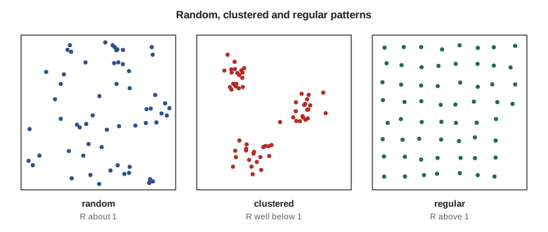
The reference model is complete spatial randomness, CSR: events occur independently, with the same probability everywhere in the window. Under CSR, counts in equal areas follow a Poisson distribution, and the distance from an event to its nearest neighbor has a known distribution. Real patterns depart from CSR in two directions. Clustered patterns have events closer together than chance, from a common cause such as a leaking reach or social contagion in reporting. Regular, or dispersed, patterns have events farther apart, as with turnouts placed at intervals or trees in an orchard.

Intensity and kernel density

Intensity is the expected number of events per unit area, λ. For a homogeneous process it is a single number, the count divided by the area. For most real processes it varies over the window, and kernel density estimation maps that variation. Each event is replaced by a smooth bump, the kernel, and the bumps are added up. The bandwidth controls the width of the bumps and dominates the result: too small and the map shows every event as a spike; too large and real clusters blur into a regional gradient. There are rules of thumb for choosing it, but the honest practice is to show the map at two or three bandwidths and say which features survive all of them.

Kernel density is a description, not a test. A hot spot on a kernel map may be no more than chance, and kernel maps of events always mirror the underlying population at risk: more complaints come from where more people farm next to the canal. Comparing a kernel map of complaints with a kernel map of the frontage of fields along the canal, as a ratio, is more informative than either alone.

Quadrat counts

The oldest test divides the window into equal cells, called quadrats, and counts events in each. Under CSR, the counts are Poisson, so their variance equals their mean. The variance-to-mean ratio, VMR, is about 1 for random patterns, greater than 1 for clustered patterns, because some cells have many events and many have none, and less than 1 for regular ones. A chi-squared test compares the observed counts with Poisson expectation. The weakness of quadrat methods is the modifiable areal unit problem again: the result depends on the size of the quadrats, and a pattern can look random at one scale and clustered at another.

Nearest neighbor distances

The Clark-Evans test uses the mean distance from each event to its nearest neighbor. Under CSR with intensity λ, the expected mean distance is one over twice the square root of λ. The ratio R of observed to expected is about 1 for randomness, below 1 for clustering, and above 1 for regularity, with a maximum of about 2.15 for a perfect hexagonal lattice. A z-score uses the standard error of the mean under CSR.

Nearest neighbor statistics see only the shortest distances, so they describe clustering at the smallest scale. Events near the edge of the window have their true nearest neighbor outside it, which inflates observed distances; the bias is small for large windows and can be reduced with a buffer zone of events counted as neighbors but not as centers.

Ripley's K and the L function

Ripley's K function looks at all scales at once. For each distance d, K(d) is the expected number of further events within d of a typical event, divided by the intensity. Under CSR, K(d) = πd². Besag's L function, the square root of K over π, turns that parabola into a straight line, L(d) = d, so that departures are easy to see: L(d) − d above zero means clustering at distance d, below zero means regularity.

Significance comes from simulation. The analyst generates many patterns of the same number of events under CSR in the same window, computes L for each, and plots the highest and lowest values at each distance as an envelope. An observed L outside the envelope is unusual under CSR. With 19 simulations the envelope corresponds to a pointwise test at about the 5 percent level in each tail combined, and with 99 simulations to the 1 percent level. Because the test is repeated at every distance, a curve that crosses the envelope briefly is weak evidence; one that stays outside over a range of distances is strong.

The code below simulates a complaint pattern on a rectangular window around a canal reach: a background of random reports plus three leaking spots that generate extra reports nearby. It computes the variance-to-mean ratio of quadrat counts, the Clark-Evans ratio and z-score, and the L function at several distances with an envelope from 19 random patterns.

import math, random
random.seed(440)
W, H = 6000.0, 1000.0                       # window around the canal reach, m
A = W * H
pts = [(random.uniform(0, W), random.uniform(0, H)) for _ in range(90)]          # background
for cx, cy, n in ((1200, 450, 25), (3400, 600, 20), (4900, 400, 15)):            # leaking spots
    pts += [(cx + random.gauss(0, 120), cy + random.gauss(0, 90)) for _ in range(n)]
pts = [(x, y) for x, y in pts if 0 <= x <= W and 0 <= y <= H]
n = len(pts); lam = n / A
print(f"events {n}, intensity {lam * 1e6:.1f} per km2")

# quadrat counts on a 12 x 2 grid of 500 m cells
counts = [0] * 24
for x, y in pts: counts[min(int(x // 500), 11) + 12 * min(int(y // 500), 1)] += 1
m = sum(counts) / 24; v = sum((c - m) ** 2 for c in counts) / 23
print(f"quadrats: mean {m:.2f}, variance {v:.2f}, VMR {v / m:.2f}")

# Clark-Evans
def nn(p, P): return min(math.dist(p, q) for q in P if q is not p)
dO = sum(nn(p, pts) for p in pts) / n
dE = 1 / (2 * math.sqrt(lam)); se = 0.26136 / math.sqrt(n * lam)
print(f"Clark-Evans: observed {dO:.1f} m, expected {dE:.1f} m, R = {dO / dE:.2f}, z = {(dO - dE) / se:.1f}")

# L function with a 19-pattern CSR envelope (no edge correction)
D = [100, 200, 400, 800]
def L(P):
    k = len(P); out = []
    for d in D:
        c = sum(1 for i in range(k) for j in range(k) if i != j and math.dist(P[i], P[j]) <= d)
        out.append(math.sqrt(A * c / (k * (k - 1)) / math.pi))
    return out
obs = L(pts)
sims = [L([(random.uniform(0, W), random.uniform(0, H)) for _ in range(n)]) for _ in range(19)]
print("   d    L(d)-d   envelope low   high")
for i, d in enumerate(D):
    lo = min(s[i] for s in sims) - d; hi = max(s[i] for s in sims) - d
    print(f"{d:5d}  {obs[i] - d:7.1f}  {lo:12.1f}  {hi:6.1f}")

events 150, intensity 25.0 per km2
quadrats: mean 6.25, variance 27.50, VMR 4.40
Clark-Evans: observed 93.9 m, expected 100.0 m, R = 0.94, z = -1.4
   d    L(d)-d   envelope low   high
  100     76.8         -14.3     7.8
  200    102.9         -21.2     0.8
  400     60.7         -60.9   -25.9
  800   -125.4        -184.7  -154.1

The tests do not all agree, and the disagreement is instructive. The variance of the quadrat counts is more than four times the mean, a clear sign of clustering at the 500 m scale. The observed L function lies above the whole envelope at every distance tested, most strongly at 100 to 200 m, about the size of the simulated leaking spots. Yet the Clark-Evans ratio is only 0.94, with a z-score of −1.4, which would not be called significant at the usual 5 percent level. The reason is that 90 of the 150 events are background reports scattered over the whole window. Their nearest neighbor distances are typical of randomness, and they dominate the mean, diluting the 60 clustered events. A statistic that sees only the closest neighbor, averaged over all events, is a weak detector of a few clusters in a random background.

Note also that the envelope is not centered on zero at the larger distances. Without edge correction, simulated random patterns in a long thin window lose neighbors across the edges, so even CSR gives L(d) below d, increasingly so as d grows toward the 1,000 m width of the window. That is why the comparison must be with simulations in the same window, not with the theoretical line. At 800 m the observed value is negative too, yet it still lies above the envelope.

The lesson Leah draws for the team is to use more than one statistic and to understand what each one sees. Quadrat counts depend on the cell size, nearest neighbor statistics see only the smallest scale and are diluted by background, and the K and L functions show the scale of clustering but need simulation for significance. When they disagree, the disagreement usually says something about the structure of the pattern.

import geopandas as gpd
from pointpats import PointPattern, k_test, l_test
import numpy as np

c = gpd.read_file("complaints.gpkg").query("category == 'seepage'")
xy = np.column_stack([c.geometry.x, c.geometry.y])
pp = PointPattern(xy)
res = l_test(xy, support=np.arange(50, 1050, 50), n_simulations=99, keep_simulations=True)
# res.support, res.statistic and res.simulations give the curve and the envelope
FIG('l03-lfun.svg', 'A chart of L(d) minus d against distance from 100 to 800 m. A shaded band shows the envelope from 19 random patterns, sloping downward with distance. The observed curve lies above the band at every distance, highest at about 200 m.', 'The observed L function lies above the simulation envelope at all distances tested.'),

Inhomogeneous processes and the population at risk

Rejecting CSR is rarely the end of the story. The complaints could be clustered simply because fields with canal frontage are clustered, or because more people live near the town end of the canal and report more. An inhomogeneous K function replaces the constant intensity with a spatially varying one, estimated from a covariate such as frontage or from a smooth trend, and tests for extra clustering beyond it. Case-control methods compare the pattern of complaints with the pattern of a control set, such as all field frontage points, and ask whether complaints cluster more than the controls do.

Leah ran both. Against a background intensity proportional to field frontage, the complaints still clustered at 200 to 500 m on three reaches, which became the candidates for the seepage investigation in the next lesson. On a fourth reach, the apparent cluster disappeared once frontage was accounted for: there were simply more fields there.

Coulee Geomatics: from dots to candidates

Leah's report to the board does not lead with the statistics. It shows the complaints map, then the same map with the three reaches outlined where clustering survives the frontage adjustment, with the distances at which it is significant. The appendix gives the window, the test, the number of simulations and the bandwidths tried. Marta asks whether a significant cluster proves a leak. It does not: it proves that complaints concentrate there more than chance and frontage explain. The next step is to look at the canal itself, with values measured along it, which needs the autocorrelation methods of lesson 4.