
GEOM-440 · Lesson 4 of 12 · 20 min
Spatial autocorrelation
Lesson 3 treated the complaints as events. The canal itself offers a different kind of data. The district's main canal is 24 km long, and for each 400 m segment the program can measure something: the number of wet-spot reports per kilometer, the rise of the water table in nearby observation wells during the irrigation season, or the share of adjoining field edges flagged as wet in the summer imagery. These are values attached to fixed spatial units, and the question becomes whether high values sit next to high values more than chance would allow, and where. That property is spatial autocorrelation, and measuring it well is central to spatial data science.
What autocorrelation is, and why it matters
Positive spatial autocorrelation means that nearby units have similar values; negative autocorrelation means neighbors tend to differ, as on a checkerboard. Most environmental variables are positively autocorrelated: soil salinity, groundwater levels, crop yield and canal seepage all vary smoothly with breaks. That is good news for prediction, because neighbors carry information, and bad news for classical statistics, because neighboring observations are not independent. A sample of 60 autocorrelated segments carries less information than 60 independent ones, so tests that assume independence report confidence that the data do not support.
Autocorrelation is also a diagnostic. If a regression model has captured the processes that drive a variable, its residuals should show little spatial pattern. Clusters of large residuals mean something spatial is missing from the model, as lesson 6 shows.
Spatial weights
Every autocorrelation statistic needs a definition of who neighbors whom, written as a spatial weights matrix W. Its element w_ij is positive if units i and j are neighbors and zero otherwise, with zeros on the diagonal. The choice of weights is part of the model and should be justified.
| Weights | Definition | Typical use |
|---|---|---|
| Rook contiguity | Polygons sharing an edge | Regular grids, townships, sections |
| Queen contiguity | Polygons sharing an edge or a corner | Irregular polygons such as fields |
| k nearest neighbors | The k closest units by centroid | Points, or polygons of uneven size |
| Distance band | All units within a distance d | Points with a known range of influence |
| Inverse distance | Weight 1/d or 1/d² up to a cutoff | Gradual influence with distance |
| Along a network | Units adjacent along a line or within a channel distance | Canals, rivers, roads |
Weights are usually row-standardized, so that each row sums to one. Then the spatially lagged value, the sum of w_ij times the neighbors' values, is simply the average of the neighbors. For the canal, the natural neighbors are the segments upstream and downstream, because seepage from one reach can raise groundwater along the next, and Leah uses the two segments on each side. Fields on opposite banks are not neighbors in this model, though they are close in straight-line distance; for the canal network, distance along the channel matters more than distance as the crow flies.
Global Moran's I
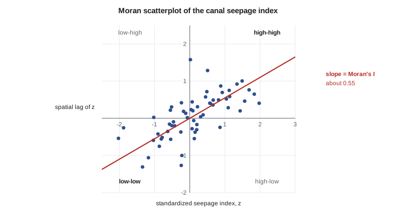
Moran's I is the most used measure of global autocorrelation. It compares each unit's deviation from the mean with its neighbors' deviations. With row-standardized weights it is close to the slope of the Moran scatterplot, which plots each unit's standardized value against the spatial lag of the standardized values.
Here S₀ is the sum of all weights, equal to n when rows are standardized. Values well above the expectation, which is slightly negative, indicate positive autocorrelation. Significance can be computed from a normal approximation, but the more robust approach is a permutation test: shuffle the values among the units many times, recompute I each time, and see where the observed I falls in that distribution. With 999 permutations, the smallest possible pseudo p-value is 0.001.
Geary's C is an alternative based on squared differences between neighbors rather than products of deviations. It is more sensitive to local differences and runs the other way: values below 1 mean positive autocorrelation. The program reports Moran's I as its headline statistic and uses Geary's C as a check.
Local indicators: LISA and hot spots
A global statistic says whether there is clustering somewhere, not where. Local indicators of spatial association, LISA, decompose the global statistic into one value per unit. The local Moran's I_i is the unit's standardized value times the lag of its neighbors. Large positive values mark high-high or low-low clusters; large negative values mark spatial outliers, high among low or low among high. Each unit's significance is tested by conditional permutation: hold the unit's own value fixed, shuffle the others among its neighbors' positions many times, and see how extreme the observed I_i is.
The Getis-Ord Gi* statistic asks a simpler question: is the sum of values in a unit's neighborhood, including the unit itself, higher or lower than expected? It is reported as a z-score, and is the basis of the hot spot analysis tools in desktop GIS. Gi* finds hot and cold spots but not outliers, so the two local statistics complement each other.
Local tests come with a serious multiple-testing problem. With 60 segments tested at the 5 percent level, three would be flagged on average even if the values were random. The program uses a stricter threshold, or a false discovery rate correction, and treats isolated significant units with suspicion unless they agree with independent evidence.
The code below builds the canal's seepage index for 60 segments, with two leaking reaches added to a smooth background, computes global Moran's I with a permutation test, and classifies each segment by local Moran with conditional permutations.
import math, random
random.seed(44)
n = 60                                         # 400 m segments along the 24 km canal
x = [1.0 + 0.4 * math.sin(i / 9.0) + random.gauss(0, 0.35) for i in range(n)]
for i in range(14, 21): x[i] += 1.6            # leaking reach near km 6 to 8
for i in range(41, 46): x[i] += 2.0            # leaking reach near km 16.5 to 18
x[33] += 2.0                                   # one isolated high reading

nb = [[j for j in (i - 2, i - 1, i + 1, i + 2) if 0 <= j < n] for i in range(n)]   # along the channel
def moran(v):
    m = sum(v) / n; z = [a - m for a in v]; s2 = sum(a * a for a in z)
    num = sum(z[i] * sum(z[j] for j in nb[i]) / len(nb[i]) for i in range(n))      # row-standardized
    return num / s2
I = moran(x)
perm = []
for _ in range(999):
    y = x[:]; random.shuffle(y); perm.append(moran(y))
p = (1 + sum(1 for v in perm if v >= I)) / 1000
print(f"Moran's I = {I:.3f}, E[I] = {-1 / (n - 1):.3f}, pseudo p = {p:.3f}")

m = sum(x) / n; sd = math.sqrt(sum((a - m) ** 2 for a in x) / n)
z = [(a - m) / sd for a in x]
def local(i, zz): return zz[i] * sum(zz[j] for j in nb[i]) / len(nb[i])
labels = []
for i in range(n):
    Ii = local(i, z); others = z[:i] + z[i + 1:]; hits = 0
    for _ in range(499):
        s = random.sample(others, len(nb[i]))
        if abs(z[i] * sum(s) / len(s)) >= abs(Ii): hits += 1
    pi = (1 + hits) / 500
    lag = sum(z[j] for j in nb[i]) / len(nb[i])
    q = ("HH" if z[i] > 0 and lag > 0 else "LL" if z[i] < 0 and lag < 0 else "HL" if z[i] > 0 else "LH")
    labels.append(q if pi <= 0.01 else ".")
print("segments 0-59, clusters at p <= 0.01:")
print("".join(f"{l:>3}" for l in labels[:30]))
print("".join(f"{l:>3}" for l in labels[30:]))
hh = [i for i, l in enumerate(labels) if l == "HH"]
print("HH segments:", hh)
print("as chainage, km:", [f"{i * 0.4:.1f}-{i * 0.4 + 0.4:.1f}" for i in hh])Moran's I = 0.545, E[I] = -0.017, pseudo p = 0.001 segments 0-59, clusters at p <= 0.01: . . . . . . . . . . . . . . . HH HH HH HH HH . . . . . . . . . . . . . . . . . . . . . . . HH . . . . . . . . . . . . . . . . HH segments: [15, 16, 17, 18, 19, 43] as chainage, km: ['6.0-6.4', '6.4-6.8', '6.8-7.2', '7.2-7.6', '7.6-8.0', '17.2-17.6']
Global Moran's I is about 0.55, far above its expectation of −0.017, and none of the 999 shuffled series came close: the seepage index is clustered along the canal. The local map is more interesting. The first leaking reach, seven segments long, shows as a run of five high-high segments from km 6.0 to 8.0. The second reach is shorter and lies where the background happens to be lowest, so at the strict 1 percent threshold only its central segment is flagged. The single high reading at segment 33 is not flagged at all, because its neighbors are ordinary: a local Moran statistic is the product of a unit's value and its neighbors' values, so an isolated spike has nothing to multiply with.
Both behaviors are the price of guarding against false positives. A strict threshold misses part of a real cluster, and a statistic built on neighbors cannot see a one-segment problem. Leah's team therefore treats the local map as a guide, not a verdict: the whole second reach goes on the field list because its central segment is flagged and the raw values are high, and segment 33 goes on it too, because a single failing culvert can leak as much as a long reach.
Autocorrelation at different scales
Moran's I depends on the weights, and so on the scale of neighborhood. A correlogram computes it for successive distance bands: neighbors within 400 m, then 400 to 800 m, and so on. For the district's real canal data, built from ten years of reports and well readings, I is high for adjacent segments, falls with distance and becomes negative beyond about 4 km, the typical length of a wet reach followed by a dry one. The distance at which the correlogram crosses zero is a rough measure of the size of the patches, and it links directly to the range of the variogram in lesson 5. It also guides the design of spatial cross-validation in lesson 7, where blocks must be larger than that distance to keep test data independent of training data.
import geopandas as gpd
from libpysal.weights import KNN
from esda.moran import Moran, Moran_Local
from esda.getisord import G_Local

seg = gpd.read_file("canal_segments.gpkg").sort_values("chainage")
w = KNN.from_dataframe(seg, k=4); w.transform = "r"      # nearest along a straight reach
mi = Moran(seg.seepage_index, w, permutations=999)
print(mi.I, mi.p_sim)
lisa = Moran_Local(seg.seepage_index, w, permutations=999, seed=44)
seg["quad"] = lisa.q; seg["p"] = lisa.p_sim                  # 1 HH, 2 LH, 3 LL, 4 HL
g = G_Local(seg.seepage_index, w, star=True, permutations=999)
seg["gi_z"] = g.Zs
Worked problem
Moran's I for five segments
Five segments in a row have values 2, 4, 5, 4, 1. Each segment's neighbors are the adjacent segments, with row-standardized weights. Compute Moran's I.
Show solution
- \[\bar x = 3.2, \qquad z = (-1.2,\ 0.8,\ 1.8,\ 0.8,\ -2.2), \qquad \textstyle\sum z^2 = 10.8\]
- \[\text{lags} = (0.8,\ 0.3,\ 0.8,\ -0.2,\ 0.8)\]
- \[\textstyle\sum z_i \cdot \text{lag}_i = -0.96 + 0.24 + 1.44 - 0.16 - 1.76 = -1.20\]
- \[I = \frac{n}{S_0}\,\frac{-1.20}{10.8} = \frac{5}{5} \times (-0.111) = -0.11\]
Answer: I ≈ −0.11, about the expectation of −0.25 under no autocorrelation for n = 5: no evidence of clustering in so short a series.
Coulee Geomatics: choosing reaches to investigate
The point pattern work in lesson 3 and the segment analysis here agree on two of the three candidate reaches. On the third, complaints cluster but the segment index does not, and the field check finds the cause: a leaking farm pipeline that runs parallel to the canal and is no concern of the district's. Marta takes the two confirmed reaches to the board with costs for lining them, and the board asks for a before-and-after design so that the effect of the lining can be measured. That request shapes lesson 10.
Common mistakes
MistakeUsing straight-line distance weights for a network such as a canal.
InsteadDefine neighbors along the channel when the process follows it.
MistakeTesting 60 local statistics at the 5 percent level and reporting every hit.
InsteadCorrect for multiple testing and confirm isolated hits independently.
MistakeReading Moran's I without its expectation and significance.
InsteadCompare with E[I] = −1/(n−1) and a permutation distribution.
MistakeTreating spatially autocorrelated observations as independent in a t-test.
InsteadAccount for autocorrelation, or the effective sample size is overstated.
Summary and key terms
- Spatial autocorrelation is the similarity of values at nearby locations.
- A spatial weights matrix defines neighbors; its choice is part of the model.
- Global Moran's I measures overall clustering; test it by permutation.
- Local Moran and Gi* locate clusters and outliers, and need multiple-testing control.
- Autocorrelation reduces effective sample size and signals missing processes in model residuals.
- For networks, measure neighborhood along the network.
- Spatial weights matrix
- A matrix whose entries say which units are neighbors and how strongly.
- Spatial lag
- The weighted average of neighbors' values.
- Moran's I
- A global statistic of spatial autocorrelation based on cross-products of deviations.
- LISA
- Local indicators of spatial association, such as local Moran's I.
- Gi*
- The Getis-Ord local statistic for hot and cold spots, reported as a z-score.
- Permutation test
- A test that compares a statistic with its values for randomly shuffled data.
Practice problems
Work each problem on paper first, then reveal the answer to check.
What is the expected value of Moran's I with no autocorrelation for 41 units?
Show answer
−1/40 = −0.025.
Why are weights row-standardized?
Show answer
So that the spatial lag is the average of the neighbors and units with many neighbors do not dominate.
What does a significant high-low LISA unit indicate?
Show answer
A high value surrounded by low values, a spatial outlier.
Why is the canal analyzed with neighbors along the channel?
Show answer
Seepage effects propagate along the canal; opposite-bank fields are not linked in that way.
Geary's C of 0.6 suggests what?
Show answer
Positive spatial autocorrelation.
Why can a local Moran statistic miss a single high segment with ordinary neighbors?
Show answer
It multiplies the unit's value by its neighbors' values, so an isolated spike has little local association to detect.
Lesson quiz · 5 questions
Score 60% or more to complete this lesson.
Create a free account to save your progress, take quizzes and earn a certificate.