Geostatistics and kriging

Salt is a slow threat on irrigated land. Where the water table rises within a couple of meters of the surface, water drawn up by evaporation leaves its dissolved salts behind, and crops lose yield long before white crusts appear. Seepage from the canal is one cause, which is why the salinity question followed the seepage one. In the spring, Grant Okonkwo's crew took 80 soil samples across a block of about 9 km² below the first leaking reach and the district's laboratory measured the electrical conductivity of a saturated paste extract, ECe, in decisiemens per meter. The board wants a map of salinity between the samples, and Leah wants an honest statement of how uncertain that map is. Kriging provides both.

From IDW to a statistical model

GEOM-330 introduced inverse distance weighting and an outline of kriging. IDW predicts a value as a weighted average of nearby samples, with weights that fall off with distance raised to a chosen power. It is simple and often adequate, but it has three weaknesses: the power is arbitrary, the weights ignore how samples cluster, so a tight group of samples gets as much influence as it has members, and it gives no measure of uncertainty. Geostatistics replaces the arbitrary weights with weights derived from a model of how the variable varies in space, fitted to the data themselves.

The model treats the variable as one realization of a random field. Under the assumption of intrinsic stationarity, the expected difference between values at two points depends only on the vector separating them, not on where the points are. The semivariogram captures that dependence: half the expected squared difference between values separated by distance h.

Reading a semivariogram

The empirical semivariogram groups all pairs of samples into distance bins and plots half the mean squared difference in each bin against the bin's mean distance. For a positively autocorrelated variable, it rises with distance and levels off. Three features describe it. The nugget is the value at very short distance, the jump at the origin, made of measurement error and variation at scales shorter than the closest sample spacing. The sill is the level where the curve flattens, about the variance of the data. The range is the distance at which it flattens: beyond the range, samples are effectively uncorrelated.

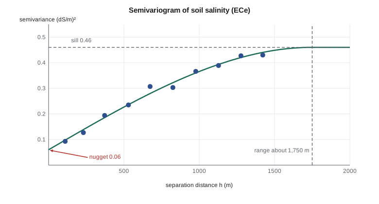
A model curve is fitted to the empirical points, because kriging needs values of γ at every distance and needs a function that guarantees valid, non-negative variances for any combination of points. Only certain functions qualify. The spherical model rises almost linearly and reaches the sill exactly at the range. The exponential model approaches the sill gradually, reaching 95 percent of it at about three times its range parameter. The Gaussian model is flat near the origin and suits very smooth variables such as some potential fields. A nugget can be added to any of them.

Fitting is usually done by weighted least squares, giving more weight to bins with many pairs and to short distances, which matter most for prediction. Bins beyond about half the maximum distance in the data have few pairs and should be ignored. Directional semivariograms, computed for pairs in a narrow range of directions, reveal anisotropy: salinity below the canal may vary more slowly along the slope than across it, which shows as a longer range in one direction.

Ordinary kriging

Ordinary kriging predicts the value at an unsampled location as a weighted sum of nearby samples, with weights chosen to make the prediction unbiased and its error variance as small as possible. The weights come from a set of linear equations built from the semivariogram: one equation per sample, plus one more, with a Lagrange multiplier μ, that forces the weights to sum to one. The left side holds γ between every pair of samples; the right side holds γ between each sample and the target.

The kriging variance is the payoff. It is small near samples and grows toward the sill in gaps, so a map of its square root shows where the prediction is weak. It depends only on the sample layout and the variogram model, not on the values themselves, so it can be computed before sampling to design a survey that keeps the error below a target everywhere. That property also means it is only as good as the model: a wrong variogram gives a confidently wrong variance.

Kriging handles clustered samples sensibly. If three samples sit almost on top of each other, the equations recognise that they carry nearly the same information and share their weight among them. With a nugget, kriging does not honor the samples exactly at short range, which is appropriate when the nugget reflects measurement error.

Checking the model by cross-validation

Leave-one-out cross-validation removes each sample in turn, predicts it from the others and compares. Two summaries matter. The root mean square error says how accurate the predictions are. The mean squared standardized error, the average of the squared error divided by the kriging variance, says whether the stated uncertainty is right: it should be close to 1. Much above 1 means the kriging variance is too optimistic; much below means it is too cautious. Comparing kriging with IDW on the same cross-validation is the fair test of whether the extra modeling earns its keep.

The code below simulates the 80 salinity samples, computes the empirical semivariogram, fits a spherical model by weighted least squares over a grid of parameters, predicts salinity at two locations with ordinary kriging using the 16 nearest samples, and compares leave-one-out errors of kriging and IDW.

import math, random
random.seed(5)
def T(A): return [list(r) for r in zip(*A)]
def mul(A, B): return [[sum(a * b for a, b in zip(r, c)) for c in zip(*B)] for r in A]
def inv(A):
    n = len(A); M = [list(map(float, r)) + [1.0 if i == j else 0.0 for j in range(n)] for i, r in enumerate(A)]
    for c in range(n):
        p = max(range(c, n), key=lambda r: abs(M[r][c])); M[c], M[p] = M[p], M[c]
        d = M[c][c]; M[c] = [x / d for x in M[c]]
        for r in range(n):
            if r != c:
                f = M[r][c]; M[r] = [x - f * y for x, y in zip(M[r], M[c])]
    return [r[n:] for r in M]
def diag(v): return [[v[i] if i == j else 0.0 for j in range(len(v))] for i in range(len(v))]
def col(v): return [[x] for x in v]
# 80 samples in a 3 km block below the leaking reach; ECe in dS/m (simulated)
bumps = [(800, 2200, 2.2, 450), (1900, 1300, 1.6, 600), (2600, 2600, 0.9, 400)]
def truth(x, y):
    return 1.2 + 0.0002 * (3000 - y) + sum(a * math.exp(-((x - bx) ** 2 + (y - by) ** 2) / (2 * r * r)) for bx, by, a, r in bumps)
S = []
for _ in range(80):
    x, y = random.uniform(0, 3000), random.uniform(0, 3000)
    S.append((x, y, truth(x, y) + random.gauss(0, 0.25)))
n = len(S)

# empirical semivariogram, 150 m bins to 1500 m
bins = [[0.0, 0.0, 0] for _ in range(10)]
for i in range(n):
    for j in range(i + 1, n):
        h = math.dist(S[i][:2], S[j][:2]); k = int(h // 150)
        if k < 10:
            b = bins[k]; b[0] += h; b[1] += 0.5 * (S[i][2] - S[j][2]) ** 2; b[2] += 1
emp = [(b[0] / b[2], b[1] / b[2], b[2]) for b in bins if b[2]]
print(" lag m  gamma   pairs")
for h, g, c in emp: print(f"{h:6.0f}  {g:5.3f}  {c:6d}")

def sph(h, c0, c, a): return c0 + c * (1.5 * h / a - 0.5 * (h / a) ** 3) if h < a else c0 + c
best = None
for c0 in [i * 0.02 for i in range(0, 16)]:
    for c in [i * 0.05 for i in range(4, 41)]:
        for a in range(400, 2001, 50):
            sse = sum(m * (g - sph(h, c0, c, a)) ** 2 / max(h, 1) for h, g, m in emp)
            if best is None or sse < best[0]: best = (sse, c0, c, a)
_, C0, CC, A = best
print(f"spherical fit: nugget {C0:.2f}, partial sill {CC:.2f}, range {A} m")
def gam(p, q): h = math.dist(p, q); return 0.0 if h == 0 else sph(h, C0, CC, A)

def ok(p, data, k=16):
    near = sorted(data, key=lambda s: math.dist(p, s[:2]))[:k]
    G = [[gam(a[:2], b[:2]) for b in near] + [1.0] for a in near] + [[1.0] * k + [0.0]]
    rhs = [[gam(a[:2], p)] for a in near] + [[1.0]]
    w = mul(inv(G), rhs)
    lam = [r[0] for r in w[:k]]; mu = w[k][0]
    z = sum(l * s[2] for l, s in zip(lam, near))
    var = sum(l * rhs[i][0] for i, l in enumerate(lam)) + mu
    return z, max(var, 0.0)
def idw(p, data, k=16, pw=2):
    near = sorted(data, key=lambda s: math.dist(p, s[:2]))[:k]
    ws = [1 / math.dist(p, s[:2]) ** pw for s in near]
    return sum(w * s[2] for w, s in zip(ws, near)) / sum(ws)

for name, p in (("near sample cluster", (850, 2150)), ("gap in the east", (2950, 300))):
    z, v = ok(p, S)
    print(f"{name:20s} OK {z:4.2f} dS/m  +/- {math.sqrt(v):.2f} (1 sd); truth {truth(*p):.2f}")

e_ok, e_idw, mse = [], [], []
for i in range(n):
    rest = S[:i] + S[i + 1:]
    z, v = ok(S[i][:2], rest); e_ok.append(z - S[i][2]); mse.append((z - S[i][2]) ** 2 / v)
    e_idw.append(idw(S[i][:2], rest) - S[i][2])
rm = lambda e: math.sqrt(sum(x * x for x in e) / len(e))
print(f"LOO RMSE: kriging {rm(e_ok):.3f}, IDW {rm(e_idw):.3f} dS/m; mean squared standardized error {sum(mse) / n:.2f}")

 lag m  gamma   pairs
   110  0.093      23
   231  0.127      64
   372  0.194      87
   530  0.235     136
   674  0.307     158
   825  0.303     185
   977  0.366     182
  1128  0.389     218
  1277  0.427     210
  1422  0.430     213
spherical fit: nugget 0.06, partial sill 0.40, range 1750 m
near sample cluster  OK 3.30 dS/m  +/- 0.37 (1 sd); truth 3.67
gap in the east      OK 1.71 dS/m  +/- 0.43 (1 sd); truth 1.83
LOO RMSE: kriging 0.332, IDW 0.384 dS/m; mean squared standardized error 0.73

Read the output against the theory. The empirical semivariogram rises from about 0.09 at the shortest lag and is still climbing slowly at 1,400 m, so the fitted spherical model puts the range at about 1,750 m, beyond the last bin used. The range is therefore poorly pinned down: the data say only that it is longer than about 1.2 km. The nugget of 0.06 is close to the variance of the measurement noise put into the simulation, 0.25² ≈ 0.06, which is what a nugget should capture.

The prediction near the cluster of samples in the north-west has a standard deviation of 0.37 dS/m, and the one in the gap at the south-east corner 0.43 dS/m. The gap is more uncertain, but by less than one might expect, because a long range lets even distant samples carry information. Both true values lie within about one standard deviation of the predictions. In cross-validation, kriging beats IDW by about 14 percent on root mean square error. The mean squared standardized error of 0.73 is below 1, so here the kriging variance is somewhat cautious: the real errors are smaller than it claims. That is common when the range is uncertain, and it is the safer direction to err in.

import numpy as np, pandas as pd
import gstools as gs
from pykrige.ok import OrdinaryKriging

s = pd.read_csv("ece_samples_2026.csv")                        # x, y in the master CRS (m); ece in dS/m
bins = np.arange(0, 1650, 150)
centres, gamma = gs.vario_estimate((s.x, s.y), s.ece, bins)
model = gs.Spherical(dim=2); model.fit_variogram(centres, gamma, nugget=True)
ok = OrdinaryKriging(s.x, s.y, s.ece, variogram_model="spherical",
                     variogram_parameters=[model.sill - model.nugget, model.len_scale, model.nugget])
gx = np.arange(0, 3000, 20.0); gy = np.arange(0, 3000, 20.0)
z, var = ok.execute("grid", gx, gy)                            # prediction and kriging variance

Beyond ordinary kriging

Several extensions matter in practice. Universal kriging, or kriging with an external drift, adds a trend: salinity may rise with proximity to the canal or fall with elevation, and the kriging is applied to the deviations from that trend. Cokriging uses a second, cheaper variable correlated with the first, such as apparent electrical conductivity from an electromagnetic induction survey towed across the fields, which gives thousands of readings for the cost of a few dozen laboratory samples. Indicator kriging predicts the probability that salinity exceeds a threshold, such as the 4 dS/m above which many crops lose yield, which is often what a decision needs. Block kriging predicts averages over areas, such as fields, which have smaller variance than point predictions.

For some decisions, a single best map is not enough. Kriging maps are smoother than reality, because they average. Conditional simulation produces many equally likely maps that honor the data and the variogram, each as rough as the real field. The area above 4 dS/m in each simulation, collected over a hundred simulations, gives a distribution for the affected area, which the smooth kriged map would understate.

Coulee Geomatics: the salinity map

The map that goes to the board shows predicted ECe in four classes, with the 4 dS/m line drawn boldly, and beside it a second map of the probability of exceeding 4 dS/m from indicator kriging. A third panel shows the kriging standard deviation, with the sample points, so that anyone can see where the map is weakest. Marta's first question is why the map is not certain where it looks clear. Leah points to the east of the block, where the nearest samples are 600 m away: the colors there are a best guess, and the standard deviation map says so. The board approves twenty more samples in the gaps and an electromagnetic induction survey for next spring, to be used as a covariate.