
GEOM-440 · Lesson 11 of 12 · 20 min
Visualization
By the end of the first year, the analytics program had produced more numbers than the board could read. The salinity work alone produced a prediction surface, a standard deviation surface, exceedance probabilities and twenty cross-validation statistics. Marta's request for the annual meeting was blunt: one page per question, readable by a grower who has never heard of kriging, and honest about what is not known. Visualization in spatial data science serves two audiences. For the analyst, it is a way of finding problems and patterns in data and models. For decision makers, it is the form in which the results arrive. This lesson covers both, with a focus on maps that show uncertainty and can be read by everyone.
Exploratory graphics for the analyst
Most visualizations are never published. They are the plots an analyst makes to check that data look as expected: histograms of each variable, scatterplots of pairs, maps of residuals, time series of a sample of pixels. Exploratory spatial data analysis links these views, so that selecting points in a scatterplot highlights them on the map, and a Moran scatterplot, as in lesson 4, shows which units drive autocorrelation. Many errors in this course would have been caught by one plot: the nodata values of lesson 2 appear as a spike at −9999 in a histogram, and swapped coordinates as dots in the wrong hemisphere.
Small multiples, a grid of the same map for different dates, variables or models with identical scales, are one of the most effective forms for both analysts and audiences. They let the eye compare, and they avoid the problems of animation, which is engaging but makes comparison hard because the earlier frames are gone.
Choosing a map type
| Data | Good choices | Watch for |
|---|---|---|
| Rates for areas, such as complaints per km of canal | Choropleth with a sequential scheme | Map rates or densities, never raw counts for unequal areas |
| Counts for areas | Proportional symbols | Overlapping symbols in dense areas |
| Continuous surfaces, such as kriged salinity | Continuous color or classed isarithmic map | Implied precision beyond the data |
| Values that diverge from a meaningful midpoint | Diverging scheme centered on the midpoint | Choosing a midpoint that is not meaningful |
| Categories, such as crops | Qualitative scheme of distinct hues | More than about eight classes |
| Flows, such as water deliveries | Flow lines with width by volume | Clutter; aggregate first |
Classification for choropleth maps, met in GEOM-330, chooses class breaks: equal intervals, quantiles, natural breaks or breaks with meaning, such as the 2, 4 and 8 dS/m thresholds of salinity classes used by agronomists. Meaningful breaks are usually best for decisions, because readers can act on them. Whatever the choice, the legend should show it, and the map should say what the colors mean in words, not only in numbers.
Color
Color carries most of the information on a thematic map, and it is easy to get wrong. A sequential scheme should change steadily in lightness from low to high, so that the order is visible even in grayscale or to a reader with a color vision deficiency. The rainbow scheme, still common in scientific software, fails that test: its lightness rises and falls, so yellow appears as a bright band that the eye reads as a feature, and red and green, which many readers cannot distinguish, carry opposite meanings. Perceptually uniform schemes, such as viridis and cividis, and the schemes in ColorBrewer, were designed to avoid those faults and are the defaults in the firm's style.
About 8 percent of men and 0.5 percent of women of northern European ancestry have some form of red-green color vision deficiency, so in any board of a dozen people, one reader may see the map differently. Simulators show how a map appears to such readers. The simplest rule is to vary lightness as well as hue, and never to rely on red against green alone.
Accessible maps
Accessibility is a legal requirement as well as good practice for many public bodies. The Web Content Accessibility Guidelines, WCAG, set criteria such as a contrast ratio of at least 4.5 to 1 between text and its background, 3 to 1 for large text and for the graphical objects needed to understand content, alternatives in text for images, and the ability to use interactive content without a mouse. In the United States, the Department of Justice's rule under Title II of the Americans with Disabilities Act requires state and local governments' web content to meet WCAG 2.1 level AA, with compliance dates in 2027 for large entities and 2028 for smaller ones, and Section 508 applies to federal agencies. The district treats its public maps as covered. For maps, that means a text description of the main findings beside each map, legends with words, sufficient contrast, patterns or labels as well as colors, and data tables that screen readers can read.
In the contrast formula, R, G and B are the color's channels converted from the sRGB values to linear light, and L₁ is the lighter of the two colors. The ratio runs from 1, for identical colors, to 21, for black on white.
Showing uncertainty
Every map in this course has an uncertainty that the reader needs. There are several ways to show it. Side-by-side maps of the estimate and its standard deviation are simple and honest, though readers must combine them in their heads. A bivariate map uses a two-dimensional color scheme, with hue or lightness for the value and saturation for certainty, so that uncertain areas look washed out. Exceedance probability maps, from indicator kriging or simulation, answer the question decision makers usually have: how likely is it that this field is above the threshold? Hatching or transparency over uncertain areas works in print and grayscale.
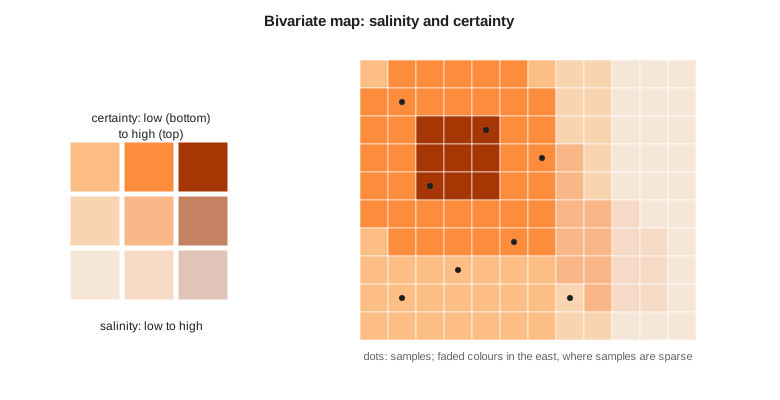
The code below computes WCAG contrast ratios for the colors in the district's map style, checks that a five-class sequential scheme rises steadily in luminance, and assigns zones to a three-by-three bivariate class from their predicted salinity and kriging standard deviation.
def lin(c):                                     # sRGB channel 0-255 to linear light
    c = c / 255
    return c / 12.92 if c <= 0.04045 else ((c + 0.055) / 1.055) ** 2.4
def lum(hexc):
    r, g, b = (int(hexc[i:i + 2], 16) for i in (1, 3, 5))
    return 0.2126 * lin(r) + 0.7152 * lin(g) + 0.0722 * lin(b)
def contrast(a, b):
    la, lb = sorted((lum(a), lum(b)), reverse=True)
    return (la + 0.05) / (lb + 0.05)

pairs = [("label text on white", "#1f2a33", "#ffffff"), ("canal line on pale field", "#3c6e9e", "#eef3e2"),
         ("gray label on pale field", "#9aa3a8", "#eef3e2"), ("white label on dark class", "#ffffff", "#7f2704")]
for name, a, b in pairs:
    r = contrast(a, b)
    print(f"{name:27s} {r:5.2f}:1  text AA {'pass' if r >= 4.5 else 'fail'}, graphics {'pass' if r >= 3 else 'fail'}")

seq = ["#fff5eb", "#fdbe85", "#fd8d3c", "#d94701", "#7f2704"]          # five salinity classes
ls = [lum(c) for c in seq]
print("luminance by class:", [round(v, 3) for v in ls], "monotonic:", all(a > b for a, b in zip(ls, ls[1:])))
rainbow = ["#0000ff", "#00ffff", "#00ff00", "#ffff00", "#ff0000"]
lr = [lum(c) for c in rainbow]
print("rainbow luminance :", [round(v, 3) for v in lr], "monotonic:", all(a > b for a, b in zip(lr, lr[1:])) or all(a < b for a, b in zip(lr, lr[1:])))

zones = [("A", 1.6, 0.20), ("B", 3.1, 0.25), ("C", 4.6, 0.22), ("D", 3.4, 0.48), ("E", 5.2, 0.45)]
def vclass(v): return 0 if v < 2.5 else 1 if v < 4.0 else 2
def uclass(s): return 0 if s < 0.3 else 1 if s < 0.4 else 2
for z, v, s in zones:
print(f"zone {z}: ECe {v:.1f} dS/m, sd {s:.2f} -> value class {vclass(v)}, certainty class {2 - uclass(s)}")label text on white 14.61:1 text AA pass, graphics pass canal line on pale field 4.74:1 text AA pass, graphics pass gray label on pale field 2.27:1 text AA fail, graphics fail white label on dark class 9.57:1 text AA pass, graphics pass luminance by class: [0.926, 0.594, 0.403, 0.193, 0.06] monotonic: True rainbow luminance : [0.072, 0.787, 0.715, 0.928, 0.213] monotonic: False zone A: ECe 1.6 dS/m, sd 0.20 -> value class 0, certainty class 2 zone B: ECe 3.1 dS/m, sd 0.25 -> value class 1, certainty class 2 zone C: ECe 4.6 dS/m, sd 0.22 -> value class 2, certainty class 2 zone D: ECe 3.4 dS/m, sd 0.48 -> value class 1, certainty class 0 zone E: ECe 5.2 dS/m, sd 0.45 -> value class 2, certainty class 0
Three of the four color pairs in the style pass easily; the gray label on the pale field color fails both the text and the graphics thresholds, at 2.3 to 1, and is replaced by a darker gray in the final style. The five-class sequential scheme falls steadily in luminance from the palest to the darkest class, so its order survives printing in grayscale. The rainbow scheme does not: its luminance jumps from dark blue to bright cyan, dips at green, peaks at yellow and falls again at red, so a reader of a grayscale copy would see the middle classes as the brightest and the highest class as darker than the middle. The bivariate classes put zones A, B and C, with small standard deviations, in the most certain row, and zones D and E, in the poorly sampled east, in the least certain row, where they will be drawn in faded colors whatever their predicted value.
A check like this takes seconds, and the firm runs it automatically on every map style before a style file is accepted. Accessibility is far easier to build in than to retrofit: a style that fails contrast after a hundred maps have been made means a hundred maps to redo.
import geopandas as gpd, matplotlib.pyplot as plt
import folium

z = gpd.read_file("salinity_zones_2026.gpkg")
fig, axes = plt.subplots(1, 3, figsize=(12, 4), constrained_layout=True)
z.plot(column="ece", cmap="cividis", scheme="user_defined", classification_kwds=dict(bins=[2, 4, 8]),
       legend=True, ax=axes[0]); axes[0].set_title("Predicted salinity (dS/m)")
z.plot(column="ece_sd", cmap="Greys", legend=True, ax=axes[1]); axes[1].set_title("Uncertainty (1 sd)")
z.plot(column="p_gt4", cmap="viridis", vmin=0, vmax=1, legend=True, ax=axes[2]); axes[2].set_title("Probability above 4 dS/m")
for a in axes: a.set_axis_off()
fig.savefig("salinity_panel.png", dpi=200)
m = z.explore(column="p_gt4", cmap="viridis", tooltip=["field_id", "ece", "ece_sd", "p_gt4"])   # interactive web map
m.save("salinity_map.html")
Interactive and web maps
Interactive maps let readers zoom, query and filter, and they suit the district's staff, who want to look up their own fields. They are not a substitute for a well-designed static map with a clear message, because readers of an interactive map may never find the part that matters. The firm publishes both: a static summary page with three maps and short text for the meeting, and an interactive map with the field table behind it for staff. Vector tiles, served from a single PMTiles file as in lesson 9, let the web map show every field quickly without a map server. Every interactive map has a keyboard-accessible table view of the same data.
Honest maps
Maps persuade, which makes them easy to misuse, deliberately or not. Choosing class breaks that exaggerate differences, a color ramp that makes a modest increase look alarming, a projection that inflates the area of interest, or a map extent that hides the context can all mislead without a single false number. The program's review checklist asks, for each map: are the breaks meaningful and shown, is the scheme ordered and accessible, is uncertainty shown, is the source and date stated, and would the message survive a different reasonable choice? If a cluster disappears with slightly different breaks, the map should not be used to claim it.
Worked problem
Contrast ratio
Text of relative luminance 0.045 sits on a background of relative luminance 0.82. Does it meet the WCAG 4.5:1 threshold for normal text?
Show solution
- \[\text{contrast} = \frac{0.82 + 0.05}{0.045 + 0.05} = \frac{0.87}{0.095}\]
- \[\text{contrast} = 9.2\]
Answer: Yes: 9.2 to 1 is well above 4.5 to 1, and above the 7 to 1 of the stricter AAA level.
Coulee Geomatics: one page per question
The annual meeting pages follow one template. A question as a heading, such as 'Where is salt building up?'. A main map with meaningful classes and a plain-language legend. A smaller uncertainty map or an exceedance map beside it. Three sentences of findings and one of limits. A footer with the data sources, dates, the method in one line and a link to the full report. All colors pass the contrast checks, all maps have text descriptions, and every map was looked at in grayscale and through a color vision simulator before it was approved. Marta's verdict after the meeting is that it was the first time growers argued about the results rather than about what the maps meant.
Common mistakes
MistakeUsing a rainbow color scheme for ordered data.
InsteadUse a perceptually uniform sequential scheme that rises steadily in lightness.
MistakeMapping raw counts for areas of different size.
InsteadMap rates or densities, or use proportional symbols for counts.
MistakeShowing an estimate without its uncertainty.
InsteadPair it with an uncertainty or exceedance map, or use a bivariate scheme.
MistakeRelying on red against green to separate classes.
InsteadVary lightness, add labels or patterns, and check with a simulator.
Summary and key terms
- Exploratory graphics catch data and model problems before they reach a report.
- Choose map types and class breaks to suit the data; meaningful breaks support decisions.
- Use perceptually ordered, color-blind-safe schemes; avoid rainbow ramps for ordered data.
- Accessible maps meet contrast thresholds, have text descriptions and do not rely on color alone.
- Show uncertainty with paired maps, bivariate schemes or exceedance probabilities.
- Review every map for misleading choices before publication.
- Choropleth map
- A map of areas shaded by the value of a variable.
- Sequential scheme
- Colors ordered from light to dark for ordered data.
- Diverging scheme
- Two sequential schemes meeting at a meaningful midpoint.
- Contrast ratio
- The WCAG measure of luminance difference between two colors.
- Bivariate map
- A map using a two-dimensional color scheme for two variables.
- Small multiples
- A grid of similar maps or charts with identical scales for comparison.
Practice problems
Work each problem on paper first, then reveal the answer to check.
Why is the rainbow scheme poor for ordered data?
Show answer
Its lightness is not monotonic, creating false bands, and it relies on red-green differences.
What contrast ratio does WCAG AA require for normal text?
Show answer
At least 4.5 to 1.
When is a diverging scheme appropriate?
Show answer
When values diverge from a meaningful midpoint, such as zero change.
What does an exceedance probability map show?
Show answer
The probability that a value is above a threshold at each location.
Why publish a static summary map as well as an interactive map?
Show answer
Readers of an interactive map may never find the key message; a static map states it.
Lesson quiz · 5 questions
Score 60% or more to complete this lesson.
Create a free account to save your progress, take quizzes and earn a certificate.