Spatial regression

With seepage and salinity mapped, the board's next question was about money: how much yield does salt cost the district's growers, and does extra irrigation water make up for it? Forty cooperating growers shared combine yield-monitor records for spring wheat, which Theo cleaned and averaged to 120 field zones of roughly 25 acres. For each zone the program has the kriged ECe from lesson 5, the water delivered through the turnout per acre, and the distance to the canal. A regression of yield on those variables looks like the obvious tool. This lesson shows why ordinary regression misleads with spatial data, and what to use instead.

Ordinary least squares and its assumptions

Ordinary least squares, OLS, fits y = Xβ + ε by minimizing the sum of squared residuals. Its estimates are unbiased if the model is correctly specified, and its standard errors are right if the errors are independent with constant variance. Spatial data break the second condition routinely and the first often. If yield is affected by something not in the model, such as soil texture or a grower's management, and that factor is itself spatially autocorrelated, the residuals inherit its pattern. Then the standard errors are too small and the significance of every coefficient is overstated. If the omitted factor is also correlated with an included variable, the coefficients themselves are biased.

The first diagnostic is Moran's I of the residuals, with a weights matrix as in lesson 4. A significant positive value says that the model leaves spatial structure unexplained. Lagrange multiplier tests, run on the OLS results, go further and indicate whether a spatial lag model or a spatial error model is more appropriate.

Spatial lag and spatial error models

The spatial lag model adds the weighted average of neighboring outcomes as a predictor. It suits processes where outcomes genuinely spill over between units: house prices influenced by neighboring prices, or yields affected by neighbors' pest pressure or shared drainage. The coefficient ρ measures the strength of the spillover. Because the lag term is correlated with the error, the model is estimated by maximum likelihood or instrumental variables, not by OLS.

The spatial error model leaves the outcome alone and puts the spatial structure in the errors. It suits the common situation where autocorrelation comes from omitted variables that vary smoothly, such as soil texture, rather than from spillovers. Its coefficient λ measures autocorrelation in the disturbance. The β estimates are then efficient and their standard errors honest.

Interpretation differs between them. In the error model, β is the effect of a unit change in x on y, as in OLS. In the lag model, a change in x in one unit affects its neighbors' y through the lag, and they in turn affect it, so the total effect is β multiplied by a factor that depends on ρ and the weights; the PySAL tools report direct, indirect and total impacts for that reason. For the yield question, there is little reason to expect yield to spill over from one zone to the next, so Leah expects the error model to fit the process better, and the tests agree.

Geographically weighted regression

Both models above assume that the relationship is the same everywhere: one β for salinity across the district. That may not hold. Salt may hurt yield more on coarse soils, which drain poorly near the water table, than on loams; water may help more where the water table is deep. Geographically weighted regression, GWR, fits a separate regression at each location, weighting observations by their distance from it with a kernel. The result is a map of each coefficient.

The bandwidth b plays the same role as in kernel density: too small, and each local regression rests on a handful of points and the coefficients swing wildly; too large, and GWR becomes OLS. It is chosen by minimizing a corrected Akaike information criterion or by cross-validation. Multiscale GWR, MGWR, allows a different bandwidth for each variable, so that a coefficient that truly varies only regionally is not forced to vary locally.

GWR has pitfalls. Local coefficients are correlated with each other, so apparent patterns in two coefficient maps can be artifacts of collinearity. The many local tests have the multiple-testing problem of lesson 4. And variation in coefficients can be caused by a missing variable rather than a real change in the relationship. GWR is best treated as an exploratory tool that suggests interactions, such as salinity times soil texture, to test in a global model.

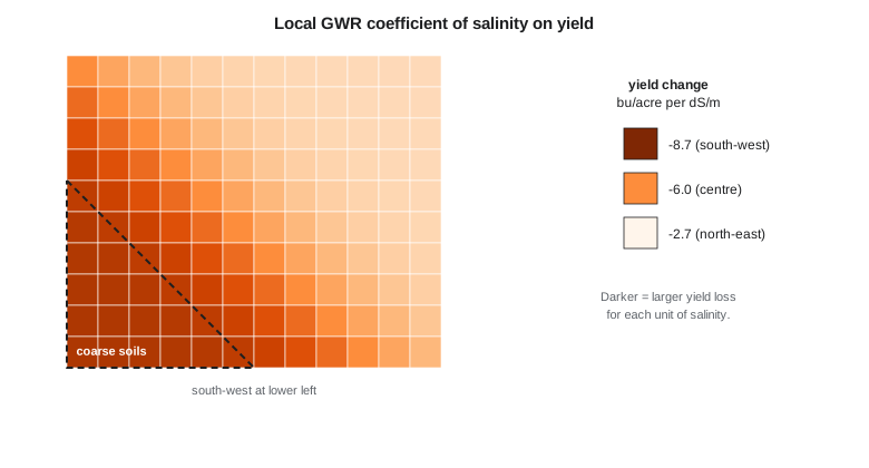
The code below simulates the 120 zones, with a salinity penalty that is stronger in the south-west and an omitted soil factor that varies smoothly. It fits OLS, tests the residuals with Moran's I, and fits GWR at three locations to show how the salinity coefficient changes.

import math, random
random.seed(66)
def T(A): return [list(r) for r in zip(*A)]
def mul(A, B): return [[sum(a * b for a, b in zip(r, c)) for c in zip(*B)] for r in A]
def inv(A):
    n = len(A); M = [list(map(float, r)) + [1.0 if i == j else 0.0 for j in range(n)] for i, r in enumerate(A)]
    for c in range(n):
        p = max(range(c, n), key=lambda r: abs(M[r][c])); M[c], M[p] = M[p], M[c]
        d = M[c][c]; M[c] = [x / d for x in M[c]]
        for r in range(n):
            if r != c:
                f = M[r][c]; M[r] = [x - f * y for x, y in zip(M[r], M[c])]
    return [r[n:] for r in M]
def diag(v): return [[v[i] if i == j else 0.0 for j in range(len(v))] for i in range(len(v))]
def col(v): return [[x] for x in v]
# 120 zones on a 12 x 10 grid of 300 m cells (simulated); yield in bu/acre
Z = []
for r in range(10):
    for c in range(12):
        x, y = 150 + 300 * c, 150 + 300 * r
        ece = max(0.5, 1.5 + 2.2 * math.exp(-((x - 900) ** 2 + (y - 2100) ** 2) / 8e5) + random.gauss(0, 0.4))
        water = random.uniform(300, 500)                          # mm delivered
        soil = 0.4 * math.sin(x / 900.0) + 0.3 * math.cos(y / 700.0)   # smooth omitted factor
        slope = -0.55 if x + y < 3000 else -0.25                  # stronger penalty in the south-west
        t = 5.2 + slope * ece + 0.0025 * (water - 400) + soil + random.gauss(0, 0.2)
        Z.append((x, y, ece, water, t * 14.87))
n = len(Z)
X = [[1.0, z[2], (z[3] - 400) / 100] for z in Z]; Y = [[z[4]] for z in Z]
b = mul(inv(mul(T(X), X)), mul(T(X), Y))
res = [Y[i][0] - sum(X[i][k] * b[k][0] for k in range(3)) for i in range(n)]
print(f"OLS: intercept {b[0][0]:.2f}, ECe {b[1][0]:+.3f} per dS/m, water {b[2][0]:+.3f} per 100 mm (about 4 in)")

# Moran's I of residuals, k = 6 nearest zones, permutation test
nb = [sorted(range(n), key=lambda j: math.dist(Z[i][:2], Z[j][:2]))[1:7] for i in range(n)]
def moran(e):
    m = sum(e) / n; d = [v - m for v in e]
    return sum(d[i] * sum(d[j] for j in nb[i]) / 6 for i in range(n)) / sum(v * v for v in d)
I = moran(res); sims = []
for _ in range(499):
    e = res[:]; random.shuffle(e); sims.append(moran(e))
print(f"residual Moran's I {I:.3f}, pseudo p {(1 + sum(s >= I for s in sims)) / 500:.3f}")

def gwr(p, bw=900.0):
    w = [math.exp(-math.dist(p, z[:2]) ** 2 / (2 * bw * bw)) for z in Z]
    XtW = [[X[i][k] * w[i] for i in range(n)] for k in range(3)]
    return mul(inv(mul(XtW, X)), mul(XtW, Y))
for name, p in (("south-west", (600, 600)), ("center", (1800, 1500)), ("north-east", (3000, 2700))):
    g = gwr(p)
    print(f"GWR at {name:10s}: ECe {g[1][0]:+.3f}, water {g[2][0]:+.3f}")

OLS: intercept 80.66, ECe -6.234 per dS/m, water +2.881 per 100 mm (about 4 in)
residual Moran's I 0.493, pseudo p 0.002
GWR at south-west: ECe -8.687, water +2.709
GWR at center    : ECe -6.029, water +2.817
GWR at north-east: ECe -2.650, water +3.176

OLS finds a salinity penalty of about 6.2 bu/acre per dS/m and a benefit of about 2.9 bu/acre for each extra 100 mm, about 4 in, of water. The residuals, though, are strongly autocorrelated, with Moran's I near 0.49 and a pseudo p-value of 0.002, the smallest possible with 499 permutations. The smooth soil factor left out of the model has moved into the residuals, and the OLS standard errors, not printed here, are too small. The three GWR fits show the salinity coefficient changing across the block, from about −8.7 bu/acre per dS/m in the south-west to −2.7 in the north-east, close to the values built into the simulation. The water coefficient barely changes, which is also what the simulation contains.

A real analysis would go on to fit the spatial error model, compare it with OLS by likelihood and AIC, and select the GWR bandwidth by AICc rather than fixing it at 900 m. The listing shows those steps with PySAL. In the firm's analysis of the real zones, the spatial error model's salinity coefficient was close to the OLS one, but its standard error was about 60 percent larger, which is exactly the correction the theory predicts when omitted factors are autocorrelated but not strongly correlated with salinity itself.

import geopandas as gpd, numpy as np
from libpysal.weights import KNN
from spreg import OLS, ML_Error
from mgwr.gwr import GWR
from mgwr.sel_bw import Sel_BW

z = gpd.read_file("yield_zones_2026.gpkg")
y = z[["yield"]].values; X = z[["ece", "water100"]].values
w = KNN.from_dataframe(z, k=6); w.transform = "r"
ols = OLS(y, X, w=w, spat_diag=True, moran=True, name_x=["ece", "water100"])
print(ols.summary)                                          # includes LM-lag and LM-error tests
err = ML_Error(y, X, w=w, name_x=["ece", "water100"]); print(err.betas.ravel(), err.lam)
coords = np.column_stack([z.geometry.centroid.x, z.geometry.centroid.y])
bw = Sel_BW(coords, y, X).search(criterion="AICc")
g = GWR(coords, y, X, bw).fit(); z["b_ece"] = g.params[:, 1]

Other ways to handle spatial structure

The lag, error and GWR models are not the only options. Spatial fixed effects add an indicator for each region, such as each lateral's service area, which absorbs differences between regions at the cost of saying nothing about them. Eigenvector spatial filtering adds, as extra predictors, a few smooth spatial patterns derived from the weights matrix, chosen to soak up residual autocorrelation; the remaining coefficients are then estimated with near-independent errors. Mixed models with a spatially correlated random effect, common in agricultural field trials, estimate the correlation structure with the same tools as the variogram of lesson 5.

Regression kriging joins this lesson to the last one. Fit a regression of salinity on covariates such as distance to the canal and electromagnetic conductivity, krige the residuals, and add the two surfaces. When the covariates explain much of the variation, the residuals have a short range and small sill and the combined map is better than kriging alone. It is the same idea as kriging with an external drift, approached from the regression side. Whatever the method, the test remains the same: do the residuals still show spatial structure, and do predictions hold up on data the model did not see?

Coulee Geomatics: what salt costs

The report to the board gives the district-wide answer from the spatial error model, with its honest confidence interval, and then the GWR map, with a caution that it suggests rather than proves. The penalty for salinity is about twice as large on the coarse soils of the south-west as elsewhere, which matches agronomic experience, and extra water does not offset it there. Marta's growers recognise the pattern. The board's decision follows from it: lining the leaking reach upstream of the south-west fields comes first, and the drainage program will target coarse soils within about a third of a mile of the canal.