Digital surface models

Two surface products were due in the same week. The hydraulic engineers needed a terrain model of the three coulee crossings to size the inverted siphons, and the construction contractor needed the volume of the first stockpile of excavated clay at the headworks, because it was being paid by the cubic meter. Both came from dense matching of photos, the corridor imagery for the crossings and a drone flight for the stockpile. Leah discovered quickly that a surface from photographs is not automatically a model of the ground. This lesson explains the kinds of elevation model, how dense image matching produces point clouds, how points are classified and filtered to the ground, how scattered points become grids and triangulated networks, how surfaces are used for contours and volumes, and how their accuracy depends on the terrain and its cover.

Surfaces and terrain

A digital surface model (DSM) describes the first surface seen from above: the tops of buildings, trees, crops, vehicles and stockpiles, as well as bare ground where nothing covers it. A digital terrain model (DTM) describes the bare ground, with buildings and vegetation removed, and is the basis of drainage, hydraulic and earthwork design. Digital elevation model (DEM) is used loosely for either, most often for bare-earth grids. The difference between a DSM and a DTM, sometimes called a normalized DSM, gives the heights of objects above the ground and is used to map buildings and canopy height.

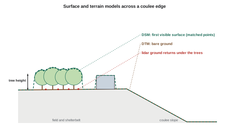
Photogrammetry measures what the camera sees. Under trees, matched points lie on the canopy; in a crop, they lie on the crop; on snow, they lie on the snow. Where the ground is hidden there is no photogrammetric measurement of it at all, and a DTM must be interpolated across the gap or supplied by lidar, which can send some pulses through gaps in the canopy to the ground. Over open prairie in late autumn, after harvest and before snow, photogrammetric surfaces can be within a few centimeters of the ground, and that is when the canal corridor was flown.

Dense image matching

Dense matching estimates a height for nearly every pixel, rather than for the thousands of tie points used in aerial triangulation. The most widely used method, semi-global matching, works on pairs of epipolar images. For each pixel in one image and each candidate disparity, a matching cost measures how dissimilar the pixel's neighborhood is from that at the corresponding position in the other image. A pure pixel-by-pixel choice of the cheapest disparity would be noisy, so the method adds penalties for changes of disparity between neighboring pixels: a small penalty for a change of one disparity step, allowing slopes, and a larger penalty for larger jumps, allowing genuine edges such as building walls but discouraging random noise. The costs are aggregated along many straight paths through the image, typically eight or sixteen directions, and the disparity with the lowest total cost is chosen.

Here \(C(\mathbf{p}, d)\) is the matching cost at pixel \(\mathbf{p}\) for disparity \(d\), \(L_r\) the cost aggregated along direction \(\mathbf{r}\), and \(P_1 < P_2\) the smoothness penalties. Disparities from many image pairs are converted to depths, checked for consistency between pairs, and fused into a point cloud. With 80 % overlap, each ground point is seen in many images, and outliers are rejected by requiring agreement among them. The point density approaches one point per GSD squared: a 10 cm GSD gives about 100 points per square meter, far more than airborne lidar typically delivers.

Matching fails or degrades where the images lack texture or change between exposures: water, shadows that move, uniform roofs, fresh snow, glass, and steep slopes seen at very different angles. It also smooths sharp features narrower than a few pixels, as Leah found at the ditch in Lesson 6. Areas hidden from one image of a pair, such as the far side of a building or the foot of a steep coulee wall, have no match and leave holes or produce wrong points at their edges.

Point clouds and classification

A point cloud is a set of points with coordinates and attributes: color from the images, the number of images that saw the point, a measure of matching quality and, after processing, a classification. The LAS format, maintained by ASPRS, is the common exchange format for both lidar and photogrammetric point clouds, and its standard classes include ground, low, medium and high vegetation, building, water, bridge deck and noise. Classification turns a DSM point cloud into a DTM by identifying the ground points.

Ground filtering algorithms exploit the fact that the ground is generally lower and smoother than the objects on it. Progressive triangulation methods start from the lowest points in a coarse grid, build a triangulated surface, and add points that lie close to it in distance and angle, iteratively densifying the ground. Morphological methods remove objects smaller than a chosen size by opening operations on a height grid. Cloth simulation methods turn the cloud upside down and drape a virtual cloth over it; the cloth settles onto the ground points. All need parameters chosen for the terrain: the steep coulee walls along the canal, which fall 60 m in a short distance, are easily mistaken for objects and cut off by a filter tuned for flat fields.

From points to surfaces

Surfaces are stored as grids or as triangulated irregular networks (TINs). A grid has heights at regular spacing, is simple to store and analyze, and is the form most software expects; its weakness is that features finer than the spacing are lost or blurred. A TIN connects the points themselves by triangles, usually a Delaunay triangulation, and interpolates linearly within each triangle; it represents variable point density and sharp features well, especially when break lines along ridges, ditches and banks are enforced as triangle edges.

Turning scattered points into a grid requires interpolation. Nearest-neighbor assignment is simple and preserves original values but produces steps. Linear interpolation in a TIN is exact at the points and continuous. Inverse distance weighting computes each grid height as a weighted average of nearby points with weights decreasing with distance,

where \(d_i\) is the distance to point \(i\) and the power \(k\) is usually 2. Kriging, from geostatistics, chooses weights from a model of how heights vary with distance and gives an estimate of the interpolation error. With the very dense clouds of photogrammetric matching, the choice of method matters less than the choice of cell size: a cell several times smaller than the point spacing invents detail, and one much larger discards it. Grids are commonly produced at one to four GSD.

Volumes

Volumes are computed as the integral of the height difference between two surfaces over an area: an original ground surface and a design or excavated surface for cut and fill, or a stockpile surface and its base. On a grid the volume is simply the sum of height differences multiplied by the cell area; on TINs it is the sum of prism volumes. The choice of base surface is often more important than the accuracy of the top: a stockpile on uneven ground may have its base defined by a pre-construction survey, by a plane through points around its toe, or by a surface interpolated beneath it, and the three can differ by several percent.

The program below simulates the headworks stockpile as a cone of radius 20 m and height 8 m, generates a dense point cloud with 3 cm noise as matching would deliver, interpolates grids at two cell sizes by inverse distance weighting, and computes the volume above the surveyed base.

# From a point cloud to a gridded surface: inverse distance weighting over a stockpile,
# then the volume above the base surface, compared with the true cone volume
import math, random
random.seed(9)

ZREF = 1010.0
base_z = ZREF + 3.20            # surveyed base of the stockpile pad (m)
R0, Hc = 20.0, 8.0              # true pile: a cone of radius 20 m and height 8 m
def truth(x, y):
    r = math.hypot(x, y)
    return base_z + max(0.0, Hc * (1 - r / R0))

# Dense matching gives scattered points with 3 cm noise (about 4 points per m2)
pts = []
for _ in range(7000):
    x, y = random.uniform(-24, 24), random.uniform(-24, 24)
    pts.append((x, y, truth(x, y) + random.gauss(0, 0.03)))

# Bin the points into 2 m cells so each grid node searches only nearby points
cells = {}
for p in pts:
    cells.setdefault((int((p[0] + 24) // 2), int((p[1] + 24) // 2)), []).append(p)

def idw(x, y, power=2.0, radius=1.5):
    i, j = int((x + 24) // 2), int((y + 24) // 2)
    num = den = 0.0
    for di in (-1, 0, 1):
        for dj in (-1, 0, 1):
            for px, py, pz in cells.get((i + di, j + dj), []):
                d = math.hypot(px - x, py - y)
                if d < 1e-6:
                    return pz
                if d <= radius:
                    w = d ** -power; num += w * pz; den += w
    return num / den if den else None

for cell in (1.0, 0.5):
    vol = 0.0; diffs = []
    n = int(48 / cell)
    for a in range(n):
        for b in range(n):
            x = -24 + (a + 0.5) * cell; y = -24 + (b + 0.5) * cell
            z = idw(x, y)
            vol += max(0.0, z - base_z) * cell * cell
            diffs.append(z - truth(x, y))
    rmse = math.sqrt(sum(d * d for d in diffs) / len(diffs))
    print(f"Grid {cell:.1f} m: {n * n:5d} nodes, RMSE against truth {100 * rmse:.1f} cm, volume {vol:8.1f} m3")
print(f"True cone volume: {math.pi * R0 ** 2 * Hc / 3:8.1f} m3")

# The effect of a base surface error: a 5 cm error over the whole pile footprint
print(f"A 5 cm error in the base surface changes the volume by {0.05 * math.pi * R0 ** 2:.0f} m3")

Grid 1.0 m:  2304 nodes, RMSE against truth 3.7 cm, volume   3354.2 m3
Grid 0.5 m:  9216 nodes, RMSE against truth 3.7 cm, volume   3354.6 m3
True cone volume:   3351.0 m3
A 5 cm error in the base surface changes the volume by 63 m3

Both grids agree with the true cone to about 0.1 %, and halving the cell size changes the volume by less than 1 m³. The small excess of about 3 m³ is a bias, not noise: around the toe of the pile, positive noise is counted as volume while negative noise below the base is clipped to zero, and the IDW average slightly rounds the apex and the toe. The last line shows the real sensitivity. A 5 cm error in the base surface over the 1257 m² footprint changes the volume by 63 m³, about 2 %, twenty times the effect of the cell size. Contractors and owners therefore agree on the base surface before the first stockpile is measured.

Contours and derived products

Contours, lines of equal elevation, are still requested for design drawings and land agreements. They are generated from a DTM grid or TIN by interpolating the positions where each contour level crosses cell edges or triangle edges and joining them. Contours from a dense matched surface are noisy and jagged; they are usually generated from a smoothed DTM or a TIN with break lines, and edited. A contour interval should be consistent with the vertical accuracy of the surface: a long-standing rule of thumb, from older map standards, relates the interval to about twice or three times the vertical error, so a surface with 10 cm vertical RMSE supports roughly a 0.25 to 0.5 m interval. Other derived products include slope and aspect grids, hillshades, flow direction and accumulation for drainage, and visibility analyses.

Accuracy of surfaces

The vertical accuracy of a surface depends on the image geometry and matching precision from Lesson 6, on the aerial triangulation, and on the terrain itself. On flat, open, textured ground, a photogrammetric surface can approach the theoretical precision. On slopes, any horizontal error becomes a vertical error equal to the horizontal error times the slope, so a 5 cm horizontal error on the 1:1 coulee wall becomes a 5 cm vertical error. In vegetation, the surface is the vegetation. Specifications therefore distinguish accuracy on non-vegetated terrain, which can be tested against checkpoints on open hard surfaces and bare ground, from accuracy in vegetated terrain, which is reported but harder to control. Lesson 12 covers how these are tested.

National and state elevation programs provide context for any project surface. The USGS 3D Elevation Program (3DEP) has collected lidar over most of the United States, typically to a quality level with about 10 cm vertical RMSE on non-vegetated ground and nominal point densities of a few points per square meter, and distributes 1 m bare-earth DEMs; Montana has extensive coverage from state and federal partnerships. A photogrammetric surface of the corridor can be compared with such data to detect gross errors, while recognizing that lidar and photogrammetry describe vegetation differently and that the two may refer to different epochs and vertical datums.

Leah's crossing models were built from the matched point cloud, filtered to the ground with parameters tuned to keep the coulee walls, combined with her compiled break lines along the drainage ditch and the old canal banks, and checked against the district's lidar of the same area. The two agreed to within 6 cm RMSE on open ground and differed by up to a meter in the shelterbelts, where only lidar had reached the ground.