
GEOM-310 · Lesson 1 of 12 · 25 min
Principles of photogrammetry
The irrigation project that commissioned the new canal west of Coulee Ridge wanted more than the control network and lidar strips that Coulee Geomatics had delivered in the fall. Its engineers needed an orthophoto of the whole 24 km corridor for the easement agreements, a surface model of the coulee crossings for the hydraulic design, a record of the old 1962 alignment from archival air photos, and regular drone surveys of the headworks during construction. Ruth Albrecht gave Leah Tran the task of explaining to the client, in plain terms, how a set of photographs becomes a measurement. This lesson is that explanation: what photogrammetry is, the geometry of a single photograph, scale and ground sample distance, relief displacement, and how the discipline grew from plane tables and glass plates to drones on a Great Falls construction site.
What photogrammetry is
Photogrammetry is the science and technology of obtaining reliable measurements of objects from their images. The word joins three Greek roots for light, writing and measuring. Its central idea is simple: a camera records the direction of the light ray from every visible point of the scene. One photograph therefore gives directions but not distances, just as a single theodolite gives angles but not positions. Two or more photographs taken from different places give intersecting directions, and intersecting directions fix points in three dimensions. Almost everything in this course is a refinement of that idea: modeling the camera precisely, finding where the camera was and how it was pointed, identifying the same point in several images, and intersecting the rays with as little error as possible.
Photogrammetry is usually divided by where the camera is. Aerial photogrammetry uses cameras in crewed aircraft or drones looking down at the ground; it produces topographic maps, orthophotos and surface models. Close-range or terrestrial photogrammetry uses cameras on the ground or on a tripod, a pole or a vehicle, at distances from a few centimeters to a few hundred meters; it measures structures, industrial parts, rock faces, accident scenes and heritage buildings. Satellite photogrammetry, covered with remote sensing in GEOM-320, uses pushbroom scanners in orbit. The geometry is the same in every case. What changes is the scale, the camera, the way the images are oriented and the accuracy that can be achieved.
Photogrammetry has two products that are easy to confuse. Metric products are coordinates: points, lines, surfaces and the maps built from them. Interpretive products describe what is in the image: land cover, crop condition, damage, vegetation. Interpretation is the domain of remote sensing and image analysis. A single project often needs both. The irrigation corridor needs metric products for design and land agreements and interpretive products for the environmental assessment of wetlands and native grassland along the route.
The geometry of a photograph
An ideal camera is a central projection. Every ray from an object point passes through a single point, the perspective center, which is the optical center of the lens, and continues to the image plane. The perpendicular from the perspective center to the image plane meets it at the principal point, and the distance between them is the principal distance, which for a camera focused at infinity equals the calibrated focal length \(f\). An aerial photograph taken with the camera pointing straight down is called a vertical photograph; in practice the camera axis is tilted by a degree or two from the vertical, and photographs deliberately tilted by more are called oblique.
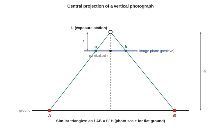
For a vertical photograph of flat ground, similar triangles give the scale directly. If the flying height above the ground is \(H\), a ground distance \(D\) appears on the photo as a distance \(d\), and
Scale is a ratio and is written as a representative fraction such as 1:20 000, read as one unit on the photo representing twenty thousand of the same units on the ground. The number after the colon is the photo scale number. Because \(H\) is the height above the ground, the scale changes wherever the ground rises or falls: on a photo taken from a fixed altitude, a hilltop is at a larger scale than a valley floor. Over the canal corridor, where the coulee rim stands 100 m above the coulee bottom, the scale varies by about 5 % within a single photo. A photograph is not a map; a map has one scale everywhere.
If the flying altitude above the vertical datum is \(H_a\) and the ground elevation is \(h\), the scale at that elevation is
Flight plans are therefore written for an average terrain elevation, and the scale or ground sample distance quoted for a project is a nominal value at that elevation.
Ground sample distance
Film cameras were described by scale. Digital cameras are described by ground sample distance (GSD), the distance on the ground between the centers of adjacent pixels. If the pixel size on the sensor is \(p\),
GSD sets the smallest detail that can be resolved, the precision of measurement, and the volume of data. It is not quite the same as resolution: blur from the lens, motion, the atmosphere and image compression mean that the smallest distinguishable feature is usually somewhat larger than one GSD, and specifications that care about detail add requirements on image sharpness. As a working rule, well-defined points can be measured to about one third to one half of a pixel in a sharp image, which is why a 10 cm GSD project can deliver horizontal accuracy of a few centimeters when its geometry and control are good.
The corridor camera has a calibrated focal length of 100 mm and a sensor of 20 000 by 13 000 pixels, each 5 µm square, mounted so that the long side is across the flight line. The district asked for a 10 cm GSD at average terrain, which fixes the flying height: \(H = \text{GSD} \cdot f / p = 0.10 \times 0.100 / 5 \times 10^{-6} = 2000\) m above the ground. The program later in the lesson works through the rest of the flight geometry.
Worked problem
Scale and GSD from a flight plan
A camera with \(f = 100\) mm and 5 µm pixels flies at 3010 m above the vertical datum over terrain whose elevation ranges from 970 m in the coulee bottoms to 1070 m on the rim, averaging 1010 m. Find the photo scale at average terrain and the GSD on the rim and in the coulee bottom.
Show solution
- \[H = 3010 - 1010 = 2000 \text{ m}, \qquad S = \frac{0.100}{2000} = \frac{1}{20\,000}\]
- \[\text{rim: } H = 3010 - 1070 = 1940 \text{ m}, \qquad \text{GSD} = \frac{5 \times 10^{-6} \times 1940}{0.100} = 0.097 \text{ m}\]
- \[\text{bottom: } H = 3010 - 970 = 2040 \text{ m}, \qquad \text{GSD} = \frac{5 \times 10^{-6} \times 2040}{0.100} = 0.102 \text{ m}\]
Answer: The scale at average terrain is 1:20 000. The GSD varies from 9.7 cm on the rim to 10.2 cm in the coulee bottoms, a spread of 5 %. A specification that demands no more than 10 cm anywhere would require flying about 40 m lower.
Relief displacement
On a vertical photograph, a point above the datum is imaged farther from the principal point than the point directly beneath it, and a point below the datum is imaged closer. The displacement is radial, away from the principal point for points above the datum. For a vertical object such as a tower, the top and the bottom are both imaged on the same radial line, and the tower appears to lean outward. Similar triangles give the relief displacement
where \(r\) is the radial distance from the principal point to the displaced image point, \(h\) is the height of the point above the reference plane and \(H\) is the flying height above that plane. Rearranged, \(h = d\,H / r\), the equation was once the standard way to measure the heights of buildings and trees from a single photograph.
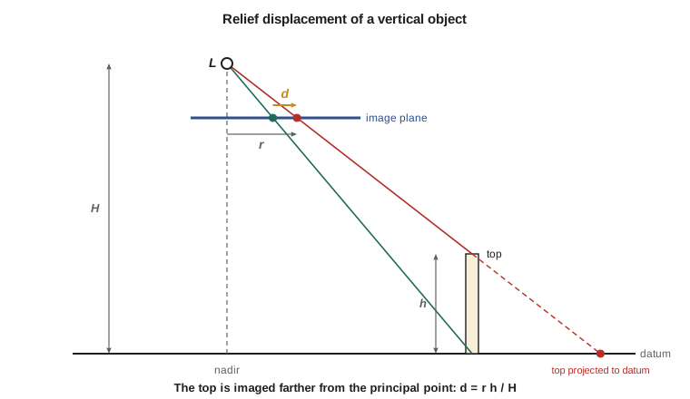
Relief displacement is both a nuisance and a signal. It is a nuisance because a photo cannot be traced as a map: every point above or below the reference plane is in the wrong place by an amount that depends on its height and its distance from the center. Removing it requires knowledge of the terrain, and that is the job of the orthophoto process in Lesson 10. It is a signal because the displacement contains the height: two photographs of the same point from different positions show different displacements, and their difference, the parallax, is the basis of stereo measurement in Lesson 6.
Relief displacement is zero at the principal point and grows linearly toward the edges of the photo. Grain elevators, bridge piers and the steep sides of the coulees all lean outward near the edges of the corridor photos. The worked numbers in the program show that a 35 m elevator imaged 45 mm from the center is displaced by about 16 m on the ground, far more than the 10 cm pixel. Any measurement from a single photograph that ignores relief is wrong by amounts of that size.
Flight geometry
Aerial photographs are taken along parallel flight lines, also called strips. Consecutive photos along a line overlap by a fraction called the forward overlap or endlap, typically 60 % for film-era mapping and 60 to 80 % for modern digital surveys. Adjacent strips overlap by the side overlap or sidelap, typically 20 to 30 % for crewed aircraft and 60 to 70 % for drones. Each area of ground must appear in at least two photos for stereo measurement; with 60 % forward overlap, a central band of each photo appears in three consecutive photos, which ties the strip together. The distance between consecutive exposure stations is the air base \(B\), and the ratio \(B/H\) controls the precision of heights.
where \(p_f\) and \(p_s\) are the forward and side overlap fractions and \(L_g\) and \(W_g\) are the ground lengths of the photo along and across the flight line. The canal corridor is narrow: the 2 km footprint across the flight line covers the 1.2 km corridor in a single strip, so no sidelap is needed except at the bends, where the strip is broken into straight segments with generous overlap at the joins.
# Photo scale, ground sample distance, coverage and relief displacement
# for the canal corridor flight
import math

ZREF = 1010.0                # average terrain elevation of the corridor (m)
f = 0.100                   # calibrated focal length (m)
pix = 5.0e-6                # pixel size on the sensor (m)
cols, rows = 20000, 13000   # sensor format in pixels: across track, along track
gsd_target = 0.10           # ground sample distance wanted at average terrain (m)

H = gsd_target * f / pix    # flying height above average terrain
alt = ZREF + H              # flying altitude above the vertical datum
print(f"Flying height above terrain   {H:8.0f} m")
print(f"Flying altitude above datum   {alt:8.0f} m")
print(f"Photo scale                   1:{H / f:,.0f}")

across, along = cols * gsd_target, rows * gsd_target
print(f"Ground footprint              {across:.0f} m x {along:.0f} m")
for overlap in (0.60, 0.80):
    base = (1 - overlap) * along
    print(f"Air base at {overlap:.0%} forward overlap  {base:6.0f} m   B/H = {base / H:.2f}")

corridor = 24000.0          # corridor length (m)
base = 0.40 * along
photos = math.ceil(corridor / base) + 1 + 2 * 2   # plus two extra photos at each end
print(f"Photos in the corridor strip  {photos}")

print()
print("GSD over the coulee relief")
for name, dz in (("coulee bottom", -40.0), ("average terrain", 0.0), ("coulee rim", 60.0)):
    h = alt - (ZREF + dz)
    print(f"  {name:16s} height above ground {h:6.0f} m   GSD {100 * pix * h / f:5.2f} cm")

print()
r = 0.045                   # radial distance of the elevator top from the principal point (m)
hgt = 35.0                  # height of a grain elevator (m)
d = r * hgt / H
print(f"Relief displacement of a {hgt:.0f} m elevator at r = {1000 * r:.0f} mm:"
f" {1000 * d:.3f} mm = {d / pix:.0f} pixels = {d * H / f:.2f} m on the ground")Flying height above terrain 2000 m Flying altitude above datum 3010 m Photo scale 1:20,000 Ground footprint 2000 m x 1300 m Air base at 60% forward overlap 520 m B/H = 0.26 Air base at 80% forward overlap 260 m B/H = 0.13 Photos in the corridor strip 52 GSD over the coulee relief coulee bottom height above ground 2040 m GSD 10.20 cm average terrain height above ground 2000 m GSD 10.00 cm coulee rim height above ground 1940 m GSD 9.70 cm Relief displacement of a 35 m elevator at r = 45 mm: 0.787 mm = 157 pixels = 15.75 m on the ground
The program confirms the hand calculation and adds the coverage numbers. With 60 % forward overlap the air base is 520 m and the base-to-height ratio 0.26; at 80 % the base halves. The 24 km strip needs about 52 photos including the extra exposures at each end, which ensure that the first and last models are complete. The relief displacement of the grain elevator, 157 pixels, shows why a photograph cannot simply be scaled and traced.
From the Rockies to the drone
Photogrammetry began almost as soon as photography. In the 1850s the French officer Aimé Laussedat used photographs taken from known stations to map terrain by intersection, and in 1867 the German architect Albrecht Meydenbauer, who measured buildings from photographs, gave the discipline its name. In North America, Édouard Deville, Surveyor General of Canada from 1885, used photo-topographic surveying to map the Rocky Mountains, where plane-table work was slow and dangerous: survey parties photographed the peaks from known summit stations and plotted the topography during the winter. In the United States, survey parties experimented with ground photographs in rugged country, and after the First World War aerial photography changed mapping completely.
Aerial photography developed rapidly after the First World War. The U.S. Geological Survey adopted aerial photographs for topographic mapping in the 1920s and 1930s, and federal agencies photographed most of the country over the following decades; the archives held by the USGS and the National Archives are the source of the photo of the 1962 canal alignment that Theo Martel ordered for Lesson 3. Through the middle of the century, mapping was done on analog stereoplotters, optical and mechanical instruments that physically recreated the geometry of the two exposures so that an operator could trace contours in a stereo model. In the late 1950s Uki Helava, working at the National Research Council of Canada, invented the analytical plotter, which replaced the mechanical linkages with a computer solving the collinearity equations in real time.
Digital photogrammetry followed in the 1980s and 1990s, first with scanned film and then with digital aerial cameras, which became standard in the 2000s. Image matching algorithms automated the measurement of tie points and surface models. In the 2010s, structure from motion, a method from computer vision that solves for camera positions and scene geometry from large sets of overlapping images with little prior information, combined with cheap drones to put photogrammetry into the hands of construction companies, farmers and archaeologists. The methods in this course span that whole history, because the geometry has not changed, and because a geomatics engineer must be able to judge the output of automated software that hides it.
Photogrammetry, lidar and surveying
Photogrammetry competes and combines with two other ways of measuring the ground. Ground surveying with total stations and GNSS, covered in GEOM-210 and GEOM-300, gives the highest accuracy at individual points but is slow over large areas. Airborne lidar, covered in GEOM-350, measures distances directly with laser pulses, penetrates gaps in vegetation to reach the ground, and works without daylight. Photogrammetry gives rich imagery, very high horizontal detail, color for interpretation, and surfaces at lower cost per square kilometer; it cannot see the ground under dense canopy and depends on light and texture.
| Method | Strength | Limitation | Typical role on the canal project |
|---|---|---|---|
| GNSS and total station | Highest point accuracy, legal survey evidence | Slow over large areas | Control and checkpoints, staking |
| Airborne lidar | Ground under vegetation, direct heights | Less image detail, cost of mobilization | Bare-earth model of the corridor |
| Aerial photogrammetry | Image detail, orthophotos, wide coverage | Needs light, texture and control | Orthophoto, planimetric mapping, coulee surface models |
| Drone photogrammetry | Low cost, flexible, very small GSD | Small areas, weather and airspace rules | Headworks construction surveys and volumes |
The skill that matters is choosing the method that meets the requirement at the lowest cost and risk, and knowing what each output can and cannot support. A surface model from photographs of a wheat field in July describes the top of the crop, not the soil; one from a December flight over stubble may be within centimeters of the ground. Knowing why is the subject of Lesson 9.
Common mistakes
MistakeTreating an aerial photograph as a map of uniform scale.
InsteadScale varies with ground elevation and with tilt; only an orthophoto has a uniform scale.
MistakeUsing flying altitude above the datum in the scale equation.
InsteadUse the height above the ground: S = f / (H_a − h).
MistakeEquating GSD with the smallest feature that can be seen.
InsteadBlur, motion and compression make the resolvable feature larger than one GSD.
MistakeMeasuring heights or positions from one photo without accounting for relief.
InsteadRelief displacement d = r h / H moves points radially; correct it or use stereo.
MistakeThinking that photogrammetry replaces ground surveying.
InsteadControl and checkpoints from ground surveys are what make photogrammetric products accurate and verifiable.
Summary and key terms
- Photogrammetry measures objects from images by intersecting light rays recorded from different positions.
- A camera is modeled as a central projection with perspective center, principal point and principal distance.
- Photo scale is f / H for a vertical photo of flat ground; it changes with terrain elevation.
- Ground sample distance GSD = p H / f sets the detail, precision and data volume of a digital survey.
- Relief displacement d = r h / H moves points radially outward; it is removed in orthophotos and exploited in stereo.
- Forward and side overlap, air base and base-to-height ratio describe the flight geometry.
- The discipline grew from ground photo-topography through analog and analytical plotters to digital and structure-from-motion methods.
- Perspective center
- The point through which all image rays pass in the central projection model of a camera.
- Principal point
- The foot of the perpendicular from the perspective center to the image plane.
- Photo scale
- The ratio of a distance on the photo to the corresponding distance on the ground.
- Ground sample distance
- The ground distance between the centers of adjacent pixels.
- Relief displacement
- The radial shift of an image point caused by its height above or below the reference plane.
- Air base
- The distance between consecutive exposure stations along a flight line.
Practice problems
Work each problem on paper first, then reveal the answer to check.
A 50 mm camera with 4 µm pixels must give a GSD of 5 cm. What flying height is needed?
Show answer
H = 0.05 × 0.050 / 4e-6 = 625 m above the ground.
A photo has scale 1:12 000. What is the ground length of a 3.5 mm photo distance?
Show answer
3.5 mm × 12 000 = 42 m.
A chimney top is imaged 78 mm from the principal point and its base 76.2 mm. The flying height is 1500 m. How tall is the chimney?
Show answer
d = 1.8 mm, h = d H / r = 1.8 × 1500 / 78 = 34.6 m.
A photo is 1300 m long on the ground in the flight direction. What is the air base for 70 % forward overlap?
Show answer
B = 0.30 × 1300 = 390 m.
Why is the scale of a photo taken over a coulee larger on the rim than in the bottom?
Show answer
The rim is closer to the camera, so H is smaller and f / H larger.
Lesson quiz · 5 questions
Score 60% or more to complete this lesson.
Create a free account to save your progress, take quizzes and earn a certificate.