Collinearity equations

Leah Tran had used the equation \(S = f / H\) for a week and was already finding its limits. The corridor photos were not exactly vertical, the ground was not flat, and the camera's position was known only from the aircraft's GNSS. Ruth told her that every serious photogrammetric computation, from orienting one photo to adjusting a block of a thousand, rests on a single pair of equations that says the perspective center, an image point and the corresponding ground point lie on one straight line. This lesson derives the collinearity equations: the rotation matrix that describes how a camera is pointed, the projection of a ground point into a photo, the inverse problem of finding a ground point from an image point, and the linearization that makes the equations usable in least squares.

The collinearity condition

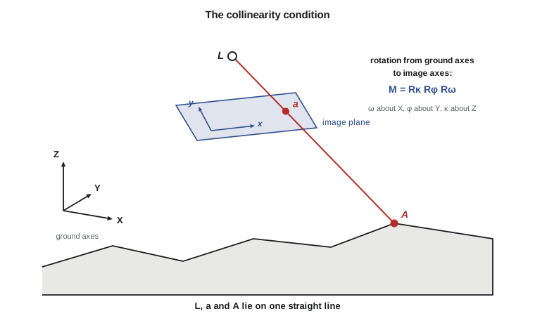
In the central projection model, the ray from a ground point \(A\) passes through the perspective center \(L\) and reaches the image plane at the image point \(a\). The three points are collinear. If the vector from \(L\) to \(A\) in ground coordinates is \((X_A - X_L,\; Y_A - Y_L,\; Z_A - Z_L)\), and the vector from \(L\) to \(a\) in image coordinates is \((x_a - x_p,\; y_a - y_p,\; -f)\), then the two vectors point in the same direction once they are expressed in the same coordinate system. Expressing the ground vector in image-space axes requires a rotation; the vectors are then proportional, with a scale factor equal to the ratio of the ground distance to the image distance.

Here \(\mathbf{M}\) is the 3 by 3 rotation matrix from ground axes to image axes and \(k\) is a scale factor that differs for every point. The six quantities \(X_L, Y_L, Z_L\) and the three angles that define \(\mathbf{M}\) are the exterior orientation of the photo: its position and attitude at the instant of exposure. Together with interior orientation from Lesson 2 they completely describe the geometry of a photograph.

The rotation matrix

Any orientation of the camera relative to the ground can be built from three rotations about coordinate axes in a fixed sequence. The traditional photogrammetric sequence uses omega (\(\omega\)) about the X axis, then phi (\(\varphi\)) about the once-rotated Y axis, then kappa (\(\kappa\)) about the twice-rotated Z axis. For a nearly vertical aerial photograph, \(\omega\) and \(\varphi\) are the small tilts across and along the flight line and \(\kappa\) is the heading of the photo's x axis relative to ground X. The individual rotation matrices are

and \(\mathbf{M} = \mathbf{R}_\kappa \mathbf{R}_\varphi \mathbf{R}_\omega\). Multiplying out gives the elements

A rotation matrix is orthogonal: its rows and columns are unit vectors at right angles, its inverse equals its transpose, \(\mathbf{M}^{-1} = \mathbf{M}^{\mathsf T}\), and its determinant is +1. These properties give a quick check on any computed matrix, and the transpose gives the rotation from image to ground axes without any inversion.

Other conventions are in common use. Inertial measurement units report roll, pitch and heading of the aircraft body, which differ from omega, phi and kappa both in sequence and in the axes they refer to; the conversion depends on how the camera is mounted, and the small boresight angles between the IMU and the camera must also be applied, as Lesson 5 explains. Computer vision usually writes the projection as \(\mathbf{x} \sim \mathbf{K}[\mathbf{R} \mid \mathbf{t}]\mathbf{X}\), with the camera looking along its positive z axis, image y downward and the focal length in pixels. The geometry is identical, but signs and axis directions differ, and confusing conventions is the most common cause of a photo that projects into the wrong quadrant or upside down.

The collinearity equations

Dividing the first and second rows of the matrix equation by the third eliminates the scale factor \(k\) and gives the collinearity equations in their usual form:

These two equations, with corrections for distortion, refraction and curvature applied to the measured image coordinates, are the mathematical model of a frame photograph. Each measured image point gives two equations. The unknowns may be the exterior orientation of the photo (space resection), the ground coordinates of the point (space intersection), or both together for many photos and points (bundle adjustment). The same equations, read from left to right, project known ground points into the photo; this is how orthophotos are made and how a surveyor checks whether a control point falls inside a given image.

For a vertical photo (\(\omega = \varphi = 0\)) of a point directly below the camera at height \(Z_A\), the equations reduce to \(x = -f(X_A - X_L)/(Z_A - Z_L)\), and since \(Z_A - Z_L = -H\) this is \(x = f(X_A - X_L)/H\): the scale equation of Lesson 1, recovered as a special case.

Projection and its inverse

The program below builds the rotation matrix for the orientation of one corridor photo, checks its orthogonality, and projects four points into it: control point CP7 near the nadir, the headgate of the new canal, a point on the coulee rim and a point on a bridge deck. It then solves the inverse problem for the headgate.

# Collinearity: project ground points into a tilted aerial photo, then intersect the ray
# of an image point with a known elevation (monoplotting)
import math

def rot(om, ph, ka):
    """Photogrammetric rotation matrix M = R3(kappa) R2(phi) R1(omega), angles in degrees."""
    o, p, k = (math.radians(a) for a in (om, ph, ka))
    so, co, sp, cp, sk, ck = math.sin(o), math.cos(o), math.sin(p), math.cos(p), math.sin(k), math.cos(k)
    return [[cp * ck, co * sk + so * sp * ck, so * sk - co * sp * ck],
            [-cp * sk, co * ck - so * sp * sk, so * ck + co * sp * sk],
            [sp, -so * cp, co * cp]]

def project(eo, P, f):
    """Collinearity: ground point P = (X, Y, Z) -> image (x, y), same units as f."""
    XL, YL, ZL, om, ph, ka = eo
    M = rot(om, ph, ka)
    d = (P[0] - XL, P[1] - YL, P[2] - ZL)
    u, v, w = (sum(M[i][j] * d[j] for j in range(3)) for i in range(3))
    return -f * u / w, -f * v / w

ZREF = 1010.0
f = 100.0                                    # focal length (mm)
eo = (10520.000, 20310.000, ZREF + 2000.0, 1.20, -0.80, 2.50)   # XL, YL, ZL (m), omega, phi, kappa (deg)
M = rot(*eo[3:])
print("Rotation matrix M")
for row in M:
    print("  " + "  ".join(f"{m:+.6f}" for m in row))
print(f"Orthogonality check: max |M M^T - I| = "
      f"{max(abs(sum(M[i][k] * M[j][k] for k in range(3)) - (i == j)) for i in range(3) for j in range(3)):.1e}")

pts = {"CP7 (nadir area)": (10500.0, 20300.0, ZREF + 12.6),
       "headgate": (11180.0, 20720.0, ZREF - 18.4),
       "coulee rim": (9840.0, 19760.0, ZREF + 61.3),
       "bridge deck": (10215.0, 20905.0, ZREF + 4.0)}
print()
print("Ground point            x (mm)      y (mm)")
img = {}
for name, P in pts.items():
    x, y = project(eo, P, f / 1000.0)
    img[name] = (1000 * x, 1000 * y)
    print(f"{name:20s} {1000 * x:10.3f}  {1000 * y:10.3f}")

# Monoplotting: from the measured image point and a known Z, solve X and Y
def monoplot(eo, x, y, Z, f):
    XL, YL, ZL = eo[:3]; M = rot(*eo[3:])
    v = [M[0][i] * x + M[1][i] * y + M[2][i] * (-f) for i in range(3)]   # ray in ground axes (M^T times image vector)
    s = (Z - ZL) / v[2]
    return XL + s * v[0], YL + s * v[1]

x, y = img["headgate"]
for dz in (0.0, 1.0):
    X, Y = monoplot(eo, x, y, pts["headgate"][2] + dz, f)
    print(f"Monoplot headgate with Z error {dz:.1f} m: X = {X:.3f}  Y = {Y:.3f}")

Rotation matrix M
  +0.998951  +0.043318  +0.014859
  -0.043615  +0.998842  +0.020314
  -0.013962  -0.020940  +0.999683
Orthogonality check: max |M M^T - I| = 2.2e-16

Ground point            x (mm)      y (mm)
CP7 (nadir area)         -2.514      -2.491
headgate                 31.789      16.690
coulee rim              -38.179     -29.164
bridge deck             -15.401      28.303
Monoplot headgate with Z error 0.0 m: X = 11180.000  Y = 20720.000
Monoplot headgate with Z error 1.0 m: X = 11179.673  Y = 20719.797

The diagonal elements of \(\mathbf{M}\) are close to 1 and the off-diagonal elements small, as they must be for a nearly vertical photo. The largest off-diagonal pair, about ±0.0434, is the sine of kappa. The orthogonality check returns a value at the level of floating-point rounding. CP7, close to the camera's nadir, projects within a few millimeters of the principal point; the coulee rim, 900 m away, projects 38 mm to the left.

Monoplotting

A single photo gives only a direction to a ground point. If the ground elevation is known from another source, such as a surface model or a design grade, the ray can be intersected with that surface, and the photo becomes a source of horizontal positions. This is monoplotting. Inverting the collinearity equations, the ray from the perspective center in ground coordinates is \(\mathbf{M}^{\mathsf T}(x, y, -f)^{\mathsf T}\), and the ground point at elevation \(Z\) is

The program recovers the headgate exactly when its true elevation is used, and shows that an elevation error of 1 m moves the result by about 0.39 m horizontally. That ratio is the tangent of the ray's angle from the vertical, here about \(r/f = 35.9 / 100\). Monoplotting is only as good as the elevation it uses, and the error grows toward the edges of the photo. This is the same relation that governs orthophoto accuracy in Lesson 10.

Linearization

The collinearity equations are nonlinear in all the unknowns: the angles appear inside sines and cosines, and the coordinates appear in a ratio. To solve them by least squares they are linearized by a Taylor series about approximate values and solved iteratively, exactly as the pseudorange equations were in GEOM-300. Writing the equations as \(x = F(\mathbf{p})\) and \(y = G(\mathbf{p})\), where \(\mathbf{p}\) contains the unknowns,

The partial derivatives with respect to the ground coordinates and the camera position are short expressions; those with respect to the angles are longer but straightforward, and textbooks tabulate them. Many modern programs compute them numerically, by changing each unknown slightly and recomputing the projection; this is simpler, avoids algebra mistakes, and is accurate enough when the step size is chosen sensibly. The programs in Lessons 5 and 7 use numerical derivatives.

Good approximate values are essential. For aerial photography they come from the flight plan or the aircraft's GNSS and inertial data: positions within tens of meters and angles within a few degrees are enough, and the iteration converges in three to five steps. For close-range or drone images taken from arbitrary directions, approximate values are harder to find, which is one reason why structure from motion begins with methods that need no approximations at all.

The coplanarity condition

Collinearity is not the only condition used in photogrammetry. The coplanarity condition states that the two perspective centers of a stereo pair and the two image points of the same ground point lie in one plane, the epipolar plane. It involves only the relative orientation of the two photos, not the ground coordinates of the point, and it is the basis of relative orientation in analytical and computer vision methods. In computer vision it appears as the essential matrix equation \(\mathbf{x}_2^{\mathsf T}\mathbf{E}\,\mathbf{x}_1 = 0\), which Lesson 8 uses to detect wrong matches.

What the equations assume

The collinearity equations describe an ideal central projection. Everything that bends the ray must be removed from the image coordinates before they are used: lens distortion, atmospheric refraction, Earth curvature where appropriate, and for film, deformation of the medium. Everything that moves the camera during exposure, such as a rolling shutter, must be modeled separately. If the corrections are incomplete, the equations still produce answers, but the residuals of the adjustment grow, and in the worst case systematic errors are absorbed silently into the exterior orientation. A good practitioner treats unexpectedly large or patterned residuals as evidence that something in the model is missing.