
GEOM-310 · Lesson 12 of 12 · 24 min
Accuracy assessment
The canal corridor deliverables were finished in March: the 10 cm orthophoto of 24 km of corridor, surface models of the three coulee crossings, the planimetric mapping, the orthophoto of the 1962 alignment and the first headworks surveys. The client's contract asked for 10 cm horizontal and 10 cm vertical accuracy, expressed as root mean square error under the ASPRS Positional Accuracy Standards, and for a statement of how it had been tested. Ruth gave the final task to Leah and Theo together: design the test, carry it out, and write the accuracy report that would go to the client with the data. This lesson draws the course together through that task: accuracy and precision, checkpoints and their selection, the statistics of positional error, current and legacy standards, testing for bias, the combination of checkpoint and product errors, and how results are reported.
Accuracy, precision and what is tested
Precision describes the internal consistency of a result, the spread of repeated measurements or the standard deviations from an adjustment. Accuracy describes closeness to the truth, which can only be judged against independent measurements of higher accuracy. The bundle adjustment of Lesson 7 reports precision; a product can be precise and still inaccurate because of a datum error, a wrong antenna height, a calibration error, or a disturbed control point. Accuracy assessment therefore compares the product with checkpoints: well-defined points, surveyed independently, that were not used to make the product.
Three kinds of accuracy are distinguished. Absolute accuracy is the agreement of coordinates with the true positions in the stated reference frame, and is what the corridor contract specifies. Relative accuracy is the agreement of distances, height differences or shapes within the dataset; it matters for design and for comparisons between surveys, such as stockpile volumes. Temporal consistency between surveys of the same site at different times is a form of relative accuracy that construction monitoring depends on. Each needs its own test: a dataset can shift by 20 cm as a whole, failing an absolute specification, while its internal geometry is excellent.
Checkpoints
A checkpoint must be well defined, identifiable without doubt in the product; independent, not used in the aerial triangulation or surface generation; accurately surveyed in the same reference frame and height system as the product; and representative, distributed over the project area and the kinds of terrain and land cover for which accuracy is claimed. For horizontal accuracy, good checkpoints are painted targets, corners of concrete pads, intersections of road markings, and the bases of utility poles, not fence posts or the edges of shadows. For vertical accuracy on open ground, checkpoints are surveyed on flat or uniformly sloping hard surfaces and short grass, away from break lines, where a small horizontal error does not become a large vertical one.
The current ASPRS standard requires at least 30 checkpoints for horizontal and non-vegetated vertical accuracy for projects up to a stated area, with more for larger projects up to a maximum of 120, and at least 30 for vegetated vertical accuracy. Thirty points give a reasonable estimate of the RMSE: the uncertainty of an RMSE estimated from \(n\) points is roughly \(\text{RMSE}/\sqrt{2n}\), about 13 % for 30 points. Fewer points give little confidence in the result, and small projects, where 30 points are impractical, report accuracy with an explicit statement of how many points were used.
The checkpoints must also be more accurate than the product. The second edition of the ASPRS standard, published in 2023 and revised in 2024, requires checkpoints at least twice as accurate as the product, relaxing the earlier requirement of three times, and requires that their own survey error be included in the final accuracy, as shown below. Grant's crew surveyed the corridor checkpoints by network RTK with repeated, independent occupations, giving about 1.5 cm horizontal and 2 cm vertical RMSE, comfortably better than the 10 cm specification.
Statistics of positional error
For each checkpoint the error is the product coordinate minus the checkpoint coordinate, \(\Delta X_i\), \(\Delta Y_i\), \(\Delta Z_i\). The summary statistics are the mean, which measures systematic error or bias; the standard deviation, which measures random spread about the mean; and the root mean square error, which combines both:
Horizontal accuracy is expressed as a single radial value, and vertical and three-dimensional values follow:
The RMSE is the measure used in current standards because it does not depend on an assumed distribution. Earlier standards converted RMSE to an accuracy at 95 % confidence by multiplying by 1.7308 horizontally, valid when the X and Y errors are similar, and by 1.9600 vertically, valid for normally distributed errors without bias. Those factors still appear in older specifications and in comparisons with legacy data.
Including the checkpoint error
Checkpoints are not perfect, and the differences between product and checkpoints contain the errors of both. When the two are independent, their variances add, and the current standard computes the product accuracy as
for each of the horizontal and vertical components. This makes the reported accuracy slightly worse than the raw comparison, which is conservative: the user is told the accuracy of the product as it would be measured against the truth, without crediting the product for errors that happened to cancel in the checkpoints. The effect is small when the checkpoints are much better than the product and large when they are only twice as good.
The corridor test
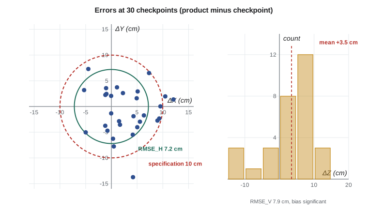
The program below analyses the 30 corridor checkpoints. It computes the statistics for each axis, the radial horizontal RMSE, the ratio of product to checkpoint accuracy, the accuracy including the checkpoint error, the three-dimensional RMSE, the comparison with the contract, the legacy 95 % values, and a test of whether the vertical mean is significantly different from zero.
# Accuracy assessment of the canal corridor orthophoto and DSM from 30 checkpoints
import math, random
random.seed(12)

n = 30
# Differences product minus checkpoint (m): small biases plus random error
dx = [0.012 + random.gauss(0, 0.045) for _ in range(n)]
dy = [-0.008 + random.gauss(0, 0.050) for _ in range(n)]
dz = [0.021 + random.gauss(0, 0.060) for _ in range(n)]

def stats(d):
    m = sum(d) / len(d)
    sd = math.sqrt(sum((x - m) ** 2 for x in d) / (len(d) - 1))
    rmse = math.sqrt(sum(x * x for x in d) / len(d))
    return m, sd, rmse
for name, d in (("X", dx), ("Y", dy), ("Z", dz)):
    m, sd, r = stats(d)
    print(f"{name}: mean {100 * m:+5.1f} cm   std dev {100 * sd:4.1f} cm   RMSE {100 * r:4.1f} cm   max |d| {100 * max(map(abs, d)):4.1f} cm")

rx, ry, rz = stats(dx)[2], stats(dy)[2], stats(dz)[2]
rh = math.hypot(rx, ry)
print(f"RMSE_H (radial) {100 * rh:.1f} cm   RMSE_V {100 * rz:.1f} cm")

# The checkpoints were surveyed by network RTK: about 1.5 cm horizontal, 2.0 cm vertical RMSE
cp_h, cp_v = 0.015, 0.020
print(f"Checkpoints are {rh / cp_h:.1f}x (horizontal) and {rz / cp_v:.1f}x (vertical) more accurate than the product")
rh_tot = math.hypot(rh, cp_h); rz_tot = math.hypot(rz, cp_v)
print(f"Product accuracy including checkpoint error: RMSE_H {100 * rh_tot:.1f} cm, RMSE_V {100 * rz_tot:.1f} cm")
rxyz = math.sqrt(rh_tot ** 2 + rz_tot ** 2)
print(f"Three-dimensional RMSE {100 * rxyz:.1f} cm")

# Against a contract that asks for 10 cm horizontal and 10 cm vertical RMSE classes
for name, val, lim in (("horizontal", rh_tot, 0.10), ("vertical", rz_tot, 0.10)):
    print(f"  {name:10s} {100 * val:4.1f} cm against {100 * lim:.0f} cm: {'meets' if val <= lim else 'fails'}")

# Older reporting at 95 % confidence (for comparison with legacy specifications)
print(f"Legacy 95 % values: horizontal {1.7308 * rh_tot * 100:.1f} cm, vertical {1.9600 * rz_tot * 100:.1f} cm")

# Is the vertical bias significant? t statistic for the mean
m, sd, _ = stats(dz)
t = m / (sd / math.sqrt(n))
print(f"Vertical mean {100 * m:+.1f} cm, t = {t:.2f} with {n - 1} degrees of freedom"
f" ({'significant' if abs(t) > 2.045 else 'not significant'} at 5 %)")X: mean +2.8 cm std dev 4.6 cm RMSE 5.3 cm max |d| 12.1 cm Y: mean -1.0 cm std dev 4.5 cm RMSE 4.5 cm max |d| 13.7 cm Z: mean +3.5 cm std dev 7.0 cm RMSE 7.7 cm max |d| 13.9 cm RMSE_H (radial) 7.0 cm RMSE_V 7.7 cm Checkpoints are 4.7x (horizontal) and 3.8x (vertical) more accurate than the product Product accuracy including checkpoint error: RMSE_H 7.2 cm, RMSE_V 7.9 cm Three-dimensional RMSE 10.7 cm horizontal 7.2 cm against 10 cm: meets vertical 7.9 cm against 10 cm: meets Legacy 95 % values: horizontal 12.4 cm, vertical 15.5 cm Vertical mean +3.5 cm, t = 2.72 with 29 degrees of freedom (significant at 5 %)
The horizontal RMSE is 7.0 cm before and 7.2 cm after including the checkpoint error, and the vertical RMSE 7.7 cm and 7.9 cm. Both meet the 10 cm specification. The checkpoints are four to five times more accurate than the product horizontally and nearly four times vertically, so including their error changes the results by only 2 to 3 mm. The legacy 95 % values, 12.4 cm horizontal and 15.5 cm vertical, are given for comparison with older data; they describe the same accuracy with a different statistic.
Testing for bias
The vertical mean error of +3.5 cm is not negligible. A t test asks whether such a mean could arise by chance from errors with zero mean: \(t = \bar{\Delta}/(s/\sqrt{n})\), compared with the critical value of Student's t distribution for \(n - 1\) degrees of freedom, 2.045 at the 5 % level for 29. Here \(t = 2.72\), so the bias is statistically significant. It does not cause the product to fail, but it is a clue: the surface is systematically about 3 cm high. Possible causes include a difference in height system or geoid model between the processing and the checkpoints, an antenna height error in the GNSS trajectory, a slight focal length error, or checkpoints surveyed on surfaces slightly lower than the matched surface, such as grass. Theo traced it to the matched surface sitting on short dormant grass at several checkpoints; on the hard-surface checkpoints alone the mean was +0.9 cm and not significant. The report states the finding.
Worked problem
Combining errors for a drone survey
A headworks DSM is tested against 30 checkpoints surveyed by RTK with an RMSE of 2.0 cm vertically. The measured vertical RMSE is 3.4 cm. Is the checkpoint survey accurate enough under the twice-as-accurate rule, and what product accuracy is reported?
Show solution
- \[\frac{3.4}{2.0} = 1.7 < 2 \quad \text{(the checkpoints are not twice as accurate)}\]
- \[\text{RMSE}_{\text{product}} = \sqrt{3.4^2 + 2.0^2} = \sqrt{11.56 + 4.00} = 3.9 \text{ cm}\]
Answer: The checkpoints fall short of the rule, and including their error raises the reported vertical accuracy from 3.4 to 3.9 cm. For centimeter-level drone products, checkpoints should be surveyed with a total station or with repeated, longer RTK occupations to reach 1 cm or better.
Standards
In the United States the ASPRS Positional Accuracy Standards for Digital Geospatial Data are the reference for photogrammetric, lidar and drone products, and federal programs such as 3DEP refer to them. The second edition, published in 2023 and revised in 2024, defines accuracy classes by RMSE alone, for example a 10 cm horizontal accuracy class, drops the 95 % confidence statistics, requires at least 30 checkpoints, relaxes the requirement for checkpoint and control accuracy to twice that of the product while including checkpoint error in the result, and adds guidance addenda for photogrammetry, lidar, drone mapping and oblique imagery. It distinguishes non-vegetated vertical accuracy, which is tested against the specification, from vegetated vertical accuracy, which is tested and reported as found.
Two older standards are still encountered. The National Map Accuracy Standards of 1947 required that 90 % of well-defined points be within 1/30 inch at map scale for maps at scales larger than 1:20 000, or 1/50 inch for smaller scales, and that 90 % of elevations be within half the contour interval; they applied to paper maps and do not translate simply to digital data. The National Standard for Spatial Data Accuracy of 1998 introduced testing with at least 20 checkpoints and reporting at 95 % confidence using the factors 1.7308 and 1.9600. Archival photography, such as the 1962 images, may have been mapped under the older standard, and comparisons with it should allow for its much looser tolerances.
| Standard | Statistic | Checkpoints | Notes |
|---|---|---|---|
| National Map Accuracy Standards (1947) | 90 % within a map-scale tolerance | Not fixed | Paper maps; 1/30 inch at large scales |
| National Standard for Spatial Data Accuracy (1998) | 95 % confidence from RMSE | At least 20 | Factors 1.7308 and 1.9600 |
| ASPRS standards, first edition (2014) | RMSE classes, also 95 % values | At least 20 | Checkpoints three times more accurate |
| ASPRS standards, second edition (2023, revised 2024) | RMSE only | At least 30, up to 120 | Checkpoints twice as accurate; their error included |
Reporting
An accuracy statement must say what was tested and how, not only the result. The corridor report stated, for each product, the accuracy class claimed, the number and distribution of checkpoints, how and when the checkpoints were surveyed and their own accuracy, the reference frame, epoch and height system, the computed RMSE values with and without checkpoint error, the means and maximum errors, the bias test, and any checkpoints excluded with the reason. A typical statement reads: tested to meet a 10 cm horizontal accuracy class, RMSE_H 7.2 cm, and a 10 cm non-vegetated vertical accuracy class, RMSE_V 7.9 cm, against 30 independent checkpoints surveyed by network RTK, with checkpoint accuracy included. The vegetated vertical accuracy in the shelterbelts and native grass along the coulee slopes was reported as found, without a pass or fail statement.
Statistics can hide patterns. A list of 30 errors with a good RMSE might have all its largest errors in one part of the corridor, near one coulee crossing or at the far end of the strip where the block was weakest. Leah plotted the errors along the corridor and as vectors on the orthophoto. The largest horizontal errors, still within tolerance, were on the steep coulee walls, as expected from Lesson 9; there was no trend along the strip, which confirmed that the control pairs and cross strips of Lesson 7 had done their job.
Accuracy of the other products
The other deliverables had their own tests. The headworks drone surveys were tested against six checkpoints per survey, too few for a formal class but enough to detect a failure, plus repeated measurements of stable points between surveys to show their relative consistency to about 2 cm. The 1962 orthophoto could not be tested against 1962 checkpoints; instead, features that had not changed since 1962, such as the corners of an old concrete headgate and section-line road intersections, were used, and the result, about 0.8 m RMSE, was reported with a description of the method and its limits. Stockpile volumes were reported with an uncertainty derived from the surface accuracy and, more importantly, the base surface agreed with the contractor.
The course in one project
The canal project used every lesson of this course. The flight geometry, GSD and relief displacement of Lesson 1 set the flight plan. The calibrated aerial camera and the self-calibrated drone camera of Lesson 2, the image coordinates and corrections of Lesson 3, and the collinearity equations of Lesson 4 described every ray. The exterior orientations of Lesson 5 came from GNSS and IMU data combined with control in the aerial triangulation of Lesson 7, while stereo measurements of Lesson 6 captured break lines. Structure from motion from Lesson 8 processed the drone flights of Lesson 11. Surfaces from Lesson 9 and orthophotos from Lesson 10 were the deliverables. The accuracy assessment of this lesson is what made them trustworthy. GEOM-350 builds on the same foundations with laser scanning and lidar, and GEOM-320 extends the imaging ideas to remote sensing from satellites.
Common mistakes
MistakeUsing control points as checkpoints.
InsteadCheckpoints must be independent of the processing; keep them separate from the start.
MistakeTesting vertical accuracy on checkpoints at break lines or in vegetation.
InsteadPlace non-vegetated vertical checkpoints on flat or uniform open surfaces; report vegetated accuracy separately.
MistakeReporting only RMSE and ignoring a significant mean.
InsteadReport the mean and test it; a significant bias points to a systematic error.
MistakeUsing checkpoints that are barely more accurate than the product.
InsteadSurvey checkpoints at least twice as accurately and include their error in the result.
MistakeConverting RMSE to 95 % values for a current specification.
InsteadThe current ASPRS edition uses RMSE only; give 95 % values only for legacy comparison.
Summary and key terms
- Precision is internal consistency; accuracy is agreement with independent, more accurate checkpoints.
- Checkpoints must be well defined, independent, accurate and representative; at least 30 are required by current standards.
- Mean, standard deviation and RMSE describe errors; RMSE_H is radial, RMSE_V vertical, RMSE_3D combined.
- Checkpoint survey error is added in quadrature to give the product accuracy.
- A t test on the mean detects bias, which points to systematic errors even when the product passes.
- The ASPRS second edition (2023, revised 2024) uses RMSE classes, 30 or more checkpoints and the twice-as-accurate rule.
- A report states what was tested, how, in which frame, and with what result, including excluded points and patterns.
- Checkpoint
- An independently surveyed, well-defined point used to test the accuracy of a product.
- Root mean square error
- The square root of the mean of squared errors, combining bias and random error.
- RMSE_H
- The radial horizontal RMSE, the square root of the sum of the squared X and Y RMSE values.
- Non-vegetated vertical accuracy
- Vertical accuracy tested on open, non-vegetated ground, used as the pass or fail criterion.
- Vegetated vertical accuracy
- Vertical accuracy in vegetated terrain, tested and reported as found.
- Bias
- A systematic error, estimated by the mean of the checkpoint differences.
Practice problems
Work each problem on paper first, then reveal the answer to check.
RMSE_X = 4 cm and RMSE_Y = 3 cm. What is RMSE_H?
Show answer
√(16 + 9) = 5 cm.
A measured vertical RMSE is 6.0 cm and the checkpoints have 1.5 cm RMSE. What product RMSE is reported?
Show answer
√(36 + 2.25) = 6.2 cm.
With 30 checkpoints, a mean of +2.0 cm and a standard deviation of 4.0 cm, is the bias significant at 5 %?
Show answer
t = 2.0 / (4.0 / √30) = 2.74 > 2.045; yes.
What 95 % horizontal value corresponds to RMSE_H = 7.0 cm under the 1998 standard?
Show answer
1.7308 × 7.0 = 12.1 cm.
Why should vertical checkpoints not be placed at the top of a canal bank?
Show answer
Small horizontal errors at a break line produce large vertical differences.
Lesson quiz · 5 questions
Score 60% or more to complete this lesson.
Create a free account to save your progress, take quizzes and earn a certificate.