
GEOM-310 · Lesson 8 of 12 · 25 min
Structure from motion
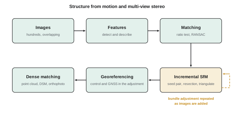
The first drone survey of the headworks produced 396 photos, no calibration report for the camera, approximate positions from the drone's own GNSS, and no attitude data worth using. The processing software asked for nothing more. It found tens of thousands of matching points, worked out where every photo had been taken, calibrated the camera, built a dense point cloud of the excavation and produced an orthophoto, all in an afternoon. Grant was impressed. Ruth was cautious: she wanted Leah to know what the software was doing, because when it went wrong it went wrong quietly. This lesson explains structure from motion, the computer vision approach behind most drone and close-range photogrammetry: feature detection and matching, robust estimation of the geometry between image pairs with the essential matrix, incremental reconstruction, the scale and datum ambiguity, georeferencing with control, and dense multi-view matching.
A different starting point
Classical aerial triangulation starts from a calibrated metric camera, a regular block of near-vertical photos, and good approximate values from the flight plan and the navigation system. Structure from motion, developed in computer vision in the 1990s and 2000s, assumes almost none of that. It accepts large numbers of overlapping images from arbitrary positions and directions, taken with cameras of unknown or approximate calibration, and recovers the camera motion, meaning the positions and orientations, together with the structure of the scene. The mathematics is the same collinearity and coplanarity geometry as Lessons 4 to 7, written in the notation of projective geometry, and the final step is always a bundle adjustment. What is different is how the solution is started, and the level of automation.
The name describes the problem: from images taken by a moving camera, recover the three-dimensional structure. In photogrammetry the method is usually combined with multi-view stereo dense matching, and the whole pipeline is sometimes called SfM-MVS. It is now the standard method for drone surveys, terrestrial photogrammetry of rock faces and structures, heritage documentation, and processing of archival photographs whose calibration has been lost.
Features and descriptors
The first step finds distinctive points in every image independently. A good feature can be located precisely and found again in another image despite changes of viewpoint, scale, rotation and lighting. Corner detectors find points where brightness changes strongly in two directions. Scale-invariant detectors search for blob-like structures across a range of image scales, so that the same feature is found whether it is imaged large or small. The best known, the scale-invariant feature transform published by David Lowe in 2004, detects extrema in a pyramid of blurred and differenced images and assigns each feature a scale and a dominant orientation.
Each feature is then described by a descriptor, a vector computed from the pattern of brightness gradients in its neighborhood, normalized for the feature's scale and orientation. The classic descriptor has 128 elements; faster binary descriptors use 256 bits; descriptors learned by neural networks are increasingly common. Descriptors of the same physical point in two images should be close; those of different points should be far apart. A typical drone image yields ten to forty thousand features.
Matching and geometric verification
Features are matched between pairs of images by comparing descriptors. For each feature in one image the nearest and second-nearest descriptors in the other are found, and the match is accepted only if the nearest is clearly closer than the second, a ratio test that rejects ambiguous matches on repetitive texture. Even so, a substantial fraction of matches are wrong, 10 to 50 % in difficult scenes. They are removed by geometric verification: correct matches must satisfy the epipolar geometry of the image pair, wrong ones in general do not.
For calibrated images, the relation between corresponding image points in normalized coordinates (image coordinates divided by the focal length) is the essential matrix equation
where \(\mathbf{R}\) and \(\mathbf{t}\) are the rotation and translation of the second camera relative to the first and \([\mathbf{t}]_\times\) is the skew-symmetric matrix that performs a cross product with \(\mathbf{t}\). This is the coplanarity condition of Lesson 4. The essential matrix has five degrees of freedom, three for rotation and two for the direction of translation; the length of the translation cannot be determined from images alone. With uncalibrated images the fundamental matrix plays the same role in pixel coordinates and has seven degrees of freedom. The essential matrix can be computed from as few as five correspondences, or more simply, with a linear algorithm, from eight.
Wrong matches are rejected with RANSAC (random sample consensus). A minimal sample of correspondences is chosen at random, a model is computed from it, and the number of other matches that agree with the model within a threshold, its inliers, is counted. After many samples the model with the most inliers is kept and re-estimated from all of them. The number of samples needed to find at least one sample free of outliers with probability \(P\), when a fraction \(w\) of matches is correct and each sample has \(s\) matches, is
Worked problem
How many RANSAC samples?
Find the number of samples needed for a 99 % chance of an outlier-free sample when 80 % of matches are correct, using the eight-point algorithm and the five-point algorithm. Repeat for 50 % correct matches.
Show solution
- \[w = 0.8, \; s = 8: \quad N = \frac{\ln 0.01}{\ln(1 - 0.8^8)} = \frac{-4.605}{\ln 0.8322} = \frac{-4.605}{-0.1837} = 25.1 \;\Rightarrow\; 26\]
- \[w = 0.8, \; s = 5: \quad N = \frac{-4.605}{\ln(1 - 0.3277)} = \frac{-4.605}{-0.3970} = 11.6 \;\Rightarrow\; 12\]
- \[w = 0.5, \; s = 8: \quad N = \frac{-4.605}{\ln(1 - 0.00391)} = 1177, \qquad s = 5: \quad N = \frac{-4.605}{\ln(1 - 0.03125)} = 145\]
Answer: Smaller minimal samples need far fewer trials, especially when many matches are wrong. This is the practical reason for preferring the five-point algorithm for calibrated cameras.
Incremental reconstruction
With verified matches for many image pairs, the reconstruction is built up step by step. An initial pair with many matches and a good baseline is chosen; its relative orientation is computed from the essential matrix, and the matched points are triangulated. New images are then added one at a time: each is oriented by resection from points already triangulated, called the perspective-n-point problem in computer vision, and its new matches are triangulated. After every few additions, a bundle adjustment refines all cameras, points and calibration parameters together, because errors would otherwise accumulate. The process continues until all images that can be connected have been added. Global methods, which estimate all rotations and then all positions at once before a final bundle adjustment, are faster for very large sets but more sensitive to wrong matches.
The result is called a sparse reconstruction: the orientations of all images, a self-calibrated camera model, and a cloud of tie points, typically tens or hundreds of thousands. Each tie point has a reprojection error, the distance between its measured image positions and the positions predicted by projecting it back into each image. The root mean square reprojection error, typically a third to one pixel, plays the same role as the reference standard deviation in aerial triangulation.
Scale, datum and the gauge
A reconstruction from images alone is determined only up to a similarity transformation: three translations, three rotations and a scale. The images would look exactly the same if the whole scene and the camera positions were moved, rotated or scaled together. In adjustment terms the problem has a seven-parameter datum defect, sometimes called the gauge freedom, and something external must fix it. In aerial triangulation the control and GNSS observations do this. In SfM the reconstruction is often first computed in an arbitrary frame, with the first camera at the origin and the first baseline of unit length, and then transformed into ground coordinates with a seven-parameter similarity transformation fitted to ground control points or to the GNSS positions of the cameras. Better practice includes the control directly in the final bundle adjustment, so that it can correct the shape of the model as well as its position.
The program below builds a miniature version of these steps for two drone images of the headgate structure, about 18 m apart and 90 m above it. It uses the known relative orientation to form the essential matrix, uses the epipolar constraint to reject wrong matches, triangulates the remaining points in a frame with a baseline of length one, and then fixes the scale from the surveyed distance between two control points.
# Structure from motion in miniature: the epipolar constraint, outlier rejection,
# triangulation in an arbitrary scale, and scaling by two ground control points
import math, random
random.seed(8)

def rot_z(deg):
    a = math.radians(deg)
    return [[math.cos(a), -math.sin(a), 0.0], [math.sin(a), math.cos(a), 0.0], [0.0, 0.0, 1.0]]
def rot_x(deg):
    a = math.radians(deg)
    return [[1.0, 0.0, 0.0], [0.0, math.cos(a), -math.sin(a)], [0.0, math.sin(a), math.cos(a)]]
def mm(A, B): return [[sum(A[i][k] * B[k][j] for k in range(3)) for j in range(3)] for i in range(3)]
def mv(A, v): return [sum(A[i][k] * v[k] for k in range(3)) for i in range(3)]
def tr(A): return [list(r) for r in zip(*A)]
def cross(a, b): return [a[1] * b[2] - a[2] * b[1], a[2] * b[0] - a[0] * b[2], a[0] * b[1] - a[1] * b[0]]
def skew(t): return [[0.0, -t[2], t[1]], [t[2], 0.0, -t[0]], [-t[1], t[0], 0.0]]

# Two drone images of the headgate structure, 18 m apart, camera looking down (z toward the ground)
f_px = 3650.0                                        # focal length in pixels
C1 = [0.0, 0.0, 0.0]; R1 = rot_x(180.0)              # world -> camera rotations
C2 = [18.0, 1.5, 0.4]; R2 = mm(rot_z(3.0), rot_x(180.0))
world = [[random.uniform(-25, 40), random.uniform(-20, 20), -random.uniform(88, 96)] for _ in range(40)]

def image(R, C, X):
    c = mv(R, [a - b for a, b in zip(X, C)])
    return [f_px * c[0] / c[2] + random.gauss(0, 0.5), f_px * c[1] / c[2] + random.gauss(0, 0.5)]
matches = [(image(R1, C1, X), image(R2, C2, X)) for X in world]
bad = random.sample(range(40), 8)                    # eight wrong matches
for k in bad:
    matches[k] = (matches[k][0], [matches[k][1][0] + random.uniform(-300, 300), matches[k][1][1] + random.uniform(-300, 300)])

# Relative orientation of camera 2 with respect to camera 1: R = R2 R1^T, t = -R (C2 - C1) * scale.
# SfM cannot know the scale, so the baseline is set to length 1.
R = mm(R2, tr(R1)); t = [-c for c in mv(R2, [b - a for a, b in zip(C1, C2)])]
n = math.sqrt(sum(c * c for c in t)); t = [c / n for c in t]
E = mm(skew(t), R)                                   # essential matrix: x2^T E x1 = 0

def ray(px): return [px[0] / f_px, px[1] / f_px, 1.0]
def sampson(x1, x2):
    Ex1 = mv(E, x1); Etx2 = mv(tr(E), x2)
    e = sum(a * b for a, b in zip(x2, Ex1))
    return e * e / (Ex1[0] ** 2 + Ex1[1] ** 2 + Etx2[0] ** 2 + Etx2[1] ** 2)

thr = (2.0 / f_px) ** 2                               # 2 pixels, squared, in normalized units
inl = [k for k, (a, b) in enumerate(matches) if sampson(ray(a), ray(b)) < thr]
print(f"{len(inl)} of {len(matches)} matches satisfy the epipolar constraint;"
      f" the {len(matches) - len(inl)} rejected include {len(set(bad) - set(inl))} of the 8 planted blunders")

# Triangulate inliers in the frame of camera 1 (midpoint of the closest approach of the rays)
c2 = mv(tr(R), [-c for c in t])                       # position of camera 2 in the camera-1 frame
def tri(a, b):
    d1 = ray(a); d2 = mv(tr(R), ray(b))
    w0 = [-c for c in c2]
    A = sum(x * x for x in d1); B = sum(x * y for x, y in zip(d1, d2)); Cc = sum(y * y for y in d2)
    D = sum(x * y for x, y in zip(d1, w0)); Ee = sum(y * z for y, z in zip(d2, w0))
    s1 = (B * Ee - Cc * D) / (A * Cc - B * B); s2 = (A * Ee - B * D) / (A * Cc - B * B)
    p1 = [s1 * x for x in d1]; p2 = [c + s2 * y for c, y in zip(c2, d2)]
    return [(u + v) / 2 for u, v in zip(p1, p2)]
model = {k: tri(*matches[k]) for k in inl}
z = [p[2] for p in model.values()]
print(f"Model depths range {min(z):.2f} to {max(z):.2f} baseline units: the shape is right, the size is not")

# Two ground control points fix the scale: their surveyed distance against the model distance
g1, g2 = inl[0], inl[-1]
d_true = math.dist(world[g1], world[g2]); d_model = math.dist(model[g1], model[g2])
s = d_true / d_model
print(f"Surveyed distance {d_true:.3f} m, model distance {d_model:.4f} units: scale {s:.3f} m per unit")
print(f"Recovered baseline {s:.3f} m (true {math.dist(C1, C2):.3f} m)")
err = []
for k, p in model.items():
    cam = mv(R1, [a - b for a, b in zip(world[k], C1)])  # true point in the camera-1 frame
    err.append(math.dist([s * c for c in p], cam))
print(f"After scaling, RMS 3D error of the {len(err)} points: {100 * math.sqrt(sum(e * e for e in err) / len(err)):.1f} cm")32 of 40 matches satisfy the epipolar constraint; the 8 rejected include 8 of the 8 planted blunders Model depths range 4.87 to 5.31 baseline units: the shape is right, the size is not Surveyed distance 51.947 m, model distance 2.8808 units: scale 18.032 m per unit Recovered baseline 18.032 m (true 18.067 m) After scaling, RMS 3D error of the 32 points: 20.3 cm
All eight planted blunders fail the epipolar test, and no correct match is rejected. The triangulated model has depths of about five baseline units: correct in shape, arbitrary in size. Two control points 52 m apart fix the scale to 18.032 m per unit, against a true baseline of 18.067 m, an error of 0.2 %. That small scale error, multiplied by depths of about 92 m, is most of the 20 cm RMS error of the scaled points. Two control points are the minimum for scale and give no check; in practice at least five well-distributed control points and independent checkpoints are used, and the control enters the bundle adjustment rather than a final transformation.
Dense matching
The sparse reconstruction describes the geometry of the cameras but not the surface in detail. Multi-view stereo dense matching then estimates a depth for nearly every pixel of every image, using the oriented images and their epipolar geometry. Methods such as semi-global matching, described in Lesson 9, and patch-based methods compare small windows along epipolar lines in several images and choose depths that are consistent between images and smooth across the surface, except at genuine edges. The depth maps are fused into a dense point cloud of tens or hundreds of millions of points, which is the raw material for surface models and orthophotos.
What can go wrong
SfM software is easy to run and hard to audit. Its typical failures are quiet. A weak block of parallel strips of near-vertical images with a self-calibrated camera can develop a bowl or dome, a smooth systematic deformation in height of decimeters over a few hundred meters, because the radial distortion and focal length are correlated with the curvature of the surface; oblique images, cross strips and good vertical control prevent it. Repetitive texture, such as rows of crops, identical roof panels or a regular formwork pattern, produces consistent wrong matches that pass the epipolar test and fold parts of the model. Moving objects, such as excavators, water surfaces and vegetation in wind, give points with no fixed position. Featureless surfaces, such as fresh snow, still water and smooth concrete, produce holes. A camera with a rolling shutter, flown fast, produces systematic errors unless its readout is modeled.
The defenses are the same as in classical photogrammetry: good geometry, a calibrated or well self-calibrated camera, sufficient well-distributed ground control, and independent checkpoints. Lesson 11 turns them into a flight plan for the headworks, and Lesson 12 describes how the results are verified and reported.
| Aspect | Classical aerial triangulation | Structure from motion |
|---|---|---|
| Camera | Metric, calibrated in the laboratory | Often consumer, self-calibrated |
| Image geometry | Regular strips of near-vertical photos | Arbitrary, often many and convergent |
| Approximate values | Flight plan, GNSS and IMU | Computed from the images |
| Tie points | Hundreds to thousands per photo, matched in epipolar geometry | Thousands per image from feature matching |
| Datum | Control and navigation data in the adjustment | Similarity transformation or control in the final adjustment |
| Final step | Bundle adjustment | Bundle adjustment |
Common mistakes
MistakeTreating SfM output as accurate because the reprojection error is small.
InsteadA small reprojection error shows internal consistency, not accuracy; check against independent checkpoints.
MistakeGeoreferencing with two or three control points by a similarity transformation.
InsteadUse enough well-distributed control in the bundle adjustment and keep checkpoints separate.
MistakeFlying only parallel vertical strips with a self-calibrated camera.
InsteadAdd oblique images or cross strips to prevent bowl and dome deformation.
MistakeTrusting matches on repetitive or moving surfaces.
InsteadMask water, moving machines and repeating patterns, and inspect the sparse cloud for folds.
MistakeAssuming the drone's own GNSS fixes the scale accurately.
InsteadNavigation-grade drone GNSS is good to meters; use RTK or PPK positions or ground control.
Summary and key terms
- Structure from motion recovers camera orientations, calibration and scene structure from overlapping images with few prior assumptions.
- Features are detected and described independently in each image and matched by comparing descriptors.
- Wrong matches are removed with RANSAC using the essential or fundamental matrix.
- Incremental reconstruction adds images by resection, triangulates points and repeats bundle adjustment.
- An image-only reconstruction has a seven-parameter datum defect that control or GNSS must fix.
- Dense multi-view matching produces point clouds for surfaces and orthophotos.
- Common failures are dome deformation, repetitive texture, moving objects and featureless surfaces.
- Structure from motion
- A method that recovers camera motion and scene structure from overlapping images.
- Feature descriptor
- A vector describing the image pattern around a detected feature, used for matching.
- Essential matrix
- A 3 by 3 matrix relating corresponding normalized image points of two calibrated cameras.
- RANSAC
- A robust estimation method that fits models to random minimal samples and keeps the one with the most inliers.
- Reprojection error
- The distance between a measured image point and the projection of its estimated ground point.
- Datum defect
- The indeterminacy of position, orientation and scale in an adjustment without external constraints.
Practice problems
Work each problem on paper first, then reveal the answer to check.
How many degrees of freedom does the essential matrix have, and why not six?
Show answer
Five: three for rotation and two for translation direction; the translation length is not determined.
With 60 % correct matches and the five-point algorithm, how many RANSAC samples give 99 % confidence?
Show answer
ln 0.01 / ln(1 − 0.6⁵) = −4.605 / −0.0809 = 57.
Why does a reconstruction need at least three non-collinear control points for a similarity transformation?
Show answer
Two points fix scale and five parameters but leave rotation about the line through them free.
What is the likely cause of a smooth 15 cm dome in a drone surface model of flat ground?
Show answer
Self-calibration correlated with surface curvature in a block of parallel vertical images.
Why are water surfaces masked before matching?
Show answer
Waves and reflections move between images, producing wrong or meaningless points.
Lesson quiz · 5 questions
Score 60% or more to complete this lesson.
Create a free account to save your progress, take quizzes and earn a certificate.