
GEOM-310 · Lesson 2 of 12 · 25 min
Cameras and calibration
Two cameras were going to work on the canal. The corridor flight would use a large-format metric aerial camera owned by an aerial survey contractor, with a calibration report signed by its manufacturer. The headworks surveys would use Coulee Geomatics' own survey drone, whose 20-megapixel camera had cost less than the fuel for one day of the crewed aircraft. Grant Okonkwo asked whether the drone camera could possibly deliver centimeter-level results. The answer depends almost entirely on calibration: on knowing the geometry of the camera well enough to reconstruct each ray as it was when the photo was taken. This lesson describes the cameras used in photogrammetry, the parameters that describe their geometry, the models for lens distortion, and the methods used to determine them.
Kinds of mapping cameras
A metric camera is one built for measurement: its lens, sensor and mount are designed to be stable, its geometry is calibrated, and the calibration is expected to hold for months or years. The classic aerial film camera exposed 230 mm by 230 mm frames behind a wide-angle lens of 152 mm focal length, with fiducial marks at the edges of the frame to define the image coordinate system. Modern large-format digital aerial cameras use either a single very large sensor or several sensors behind several lenses whose images are stitched into one virtual frame during processing. Medium-format cameras with sensors of 50 to 150 megapixels serve smaller aircraft and corridor work. A non-metric camera is a consumer or industrial camera not designed for measurement; its geometry may be excellent, but it is not guaranteed stable, and it must be calibrated in place, usually as part of each project.
Not all mapping sensors are frame cameras. Pushbroom scanners have one or a few lines of detectors across the flight direction and build the image line by line as the platform moves; they are standard on Earth observation satellites and some airborne systems. Their geometry changes with every line, so they need continuous position and attitude data and different equations from those used for frame cameras. Oblique camera systems combine a vertical camera with four cameras tilted forward, backward, left and right, and are widely used to model city façades and to produce the inclined views found in municipal viewing applications. Multispectral and thermal cameras, used for crop monitoring and building inspection, follow the same geometric principles but have larger pixels and often weaker geometry.
Sensors, shutters and motion
Digital cameras use CCD or CMOS sensors. Most color sensors carry a Bayer filter, a mosaic of red, green and blue filters over individual pixels, and each pixel's missing colors are interpolated from its neighbors. Some aerial cameras capture a sharper panchromatic image and lower-resolution color bands and combine them by pan-sharpening; others capture red, green, blue and near-infrared at full resolution. Radiometric depth is typically 12 to 14 bits per band, which preserves detail in shadows and bright concrete that an 8-bit image would lose. The pixel size of large aerial sensors is typically between about 3.5 and 6 µm.
The shutter matters to geometry. A central (leaf) shutter in the lens exposes the whole frame at once; all pixels share one exposure time and one camera position. A global electronic shutter has the same effect. A rolling shutter reads the sensor row by row, so the top and bottom of the image are exposed a few tens of milliseconds apart; if the camera moves during that interval, each row has a slightly different position, and the image is distorted in a way the central projection model does not describe. Survey drones should have mechanical or global shutters, and when they do not, processing software must model the rolling-shutter motion explicitly. Lesson 11 returns to this.
An aircraft moving at 70 m/s with a 1/1000 s exposure moves 7 cm during the exposure, enough to blur a 10 cm pixel noticeably. Aerial cameras counter this with forward motion compensation, which shifts the image during exposure to follow the ground, either mechanically for film or electronically for sensors by time-delayed integration that moves the accumulated charge across the sensor in step with the image. Gyro-stabilized mounts keep the camera close to vertical and cancel the aircraft's vibration. Drones fly much more slowly but at much smaller GSD, so blur is still a constraint on their flight speed.
Interior orientation
Interior orientation is the set of parameters that describes the geometry inside the camera: how image coordinates relate to rays through the perspective center. For an ideal central projection it has three parameters: the principal distance \(f\) (usually called the calibrated focal length) and the image coordinates of the principal point \(x_p, y_p\). For a real lens it adds parameters for lens distortion and, for some sensors, for differences in scale between the two image axes or for non-perpendicular axes. With interior orientation known, every measured image point defines a ray in the camera's own coordinate system, and the camera becomes a precise direction-measuring instrument, much like a theodolite with a field of view of 70° or more.
The principal point is not necessarily at the center of the sensor: manufacturing tolerances place the optical axis some micrometers or tens of micrometers away from the geometric center. The calibrated focal length differs slightly from the nominal focal length engraved on the lens. In older practice the principal point of best symmetry and the point of autocollimation were also distinguished; modern calibrations usually report a single principal point and a distortion model referred to it.
Lens distortion
A real lens does not bend every ray exactly through a single point. The departures are described as distortion, the displacement of the imaged point from where the ideal central projection would put it. The standard model, developed by Duane Brown in the 1960s and 1970s from earlier work by Conrady, separates two kinds. Radial distortion displaces points along radial lines from the principal point; barrel distortion moves them inward, toward the center, and pincushion distortion outward. It is modeled by an odd polynomial in the radial distance \(r\):
where \(\bar{x} = x - x_p\) and \(\bar{y} = y - y_p\) are image coordinates reduced to the principal point and \(r^2 = \bar{x}^2 + \bar{y}^2\). Decentering distortion arises when the elements of a compound lens are not perfectly centered on one axis; it has both radial and tangential components and is modeled with two coefficients:
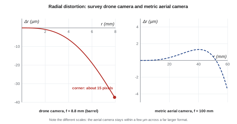
For a large-format metric aerial camera the distortion is small, a few micrometers at most, and well determined. For a consumer camera with a short wide-angle lens it may reach tens of pixels at the corners. Because distortion is systematic, its size is not the problem; an uncalibrated or wrongly calibrated distortion is. A residual error of one pixel at the edge of every photo propagates through the whole block and shows up as a bowl or dome in the surface model, a well-known symptom of drone projects processed without good calibration and without enough control.
Software packages express distortion in different units and sign conventions. Some apply the model to the observed coordinates to obtain corrected ones; others, especially in computer vision, apply it to the ideal coordinates to predict the observed ones, and use normalized coordinates (divided by the focal length) or pixels instead of millimeters. Coefficients from one convention cannot be pasted into another without conversion. When a calibration report is transferred into processing software, the safe test is to compute the distortion at a few radial distances in both and compare them.
Determining the parameters
Laboratory calibration measures the camera on an optical bench. Multicollimator and goniometer methods send collimated beams or view a precise target through the lens at known angles and measure where they are imaged; the result is the calibrated focal length, principal point and distortion curve. This was the standard for film mapping cameras and is still how manufacturers calibrate large-format digital cameras, often supplemented by flights over calibration ranges with many surveyed targets.
Test-field calibration photographs a set of precisely surveyed targets, a calibration range, from several positions and angles, and solves for the interior orientation as unknowns in a bundle adjustment. Self-calibration does the same with the project's own photographs: the interior orientation parameters are added to the unknowns of the aerial triangulation in Lesson 7. It works well when the block has strong geometry, such as convergent images, varying flying heights, and cross strips, and it is the normal method for drone cameras. In the United States the USGS calibrated film mapping cameras for decades and later ran a quality assurance program for digital aerial sensors, and federal and state contracts typically require a current calibration report and verification of the camera geometry in the project adjustment.
Self-calibration has a price. The interior orientation parameters correlate with the exterior orientation and with the shape of the block. With a flat block of vertical photos taken from one height, the focal length is almost perfectly correlated with the flying height: a camera with a slightly longer focal length at a slightly greater height produces the same photos. The adjustment then cannot separate them, and an error in focal length becomes an error in every height. Convergent or oblique images, a range of flying heights, and accurate GNSS positions of the camera, together with well-distributed ground control, break the correlation. This is why careful drone flight plans include cross strips flown at a different height or with the camera tilted.
Stability and the drone camera
A calibration describes the camera at the time it was determined. Focusing changes the principal distance, so survey cameras are fixed at infinity focus. Temperature changes the lens and the sensor mount; an aircraft at 3000 m on a February morning over the prairies is a very different environment from the calibration laboratory, and large aerial cameras are built and heated to limit the effect. Zoom lenses, automatic focus, image stabilization that moves the sensor, and in-camera distortion correction all undermine the stability of consumer cameras. A drone used for mapping should have its focus fixed, stabilization and automatic corrections disabled, and its calibration refined in every project.
The program below uses a calibration of the drone camera to show what the parameters mean in practice: the size of radial distortion across the format, the shift of a corner point, the smaller decentering part, and the conversion of a pixel position to image coordinates relative to the principal point. Removing distortion requires inverting the model, which has no closed form; a few fixed-point iterations are enough.
# Brown-Conrady lens distortion for the survey drone camera, and its removal
import math

f = 8.80                     # calibrated focal length (mm)
pix = 0.00241                # pixel size (mm)
xp, yp = 0.012, -0.018       # principal point offset from the middle of the sensor (mm)
k1, k2, k3 = -1.05e-4, 4.8e-7, 0.0     # radial coefficients (mm^-2, mm^-4, mm^-6)
p1, p2 = 2.1e-5, -1.3e-5               # decentring coefficients (mm^-1)

def distort(x, y):
    """Ideal (undistorted) image coordinates -> observed (distorted) coordinates, in mm."""
    r2 = x * x + y * y
    radial = k1 * r2 + k2 * r2 ** 2 + k3 * r2 ** 3
    dx = x * radial + p1 * (r2 + 2 * x * x) + 2 * p2 * x * y
    dy = y * radial + p2 * (r2 + 2 * y * y) + 2 * p1 * x * y
    return x + dx, y + dy

def undistort(xd, yd, n=10):
    """Invert the model by fixed-point iteration."""
    x, y = xd, yd
    for _ in range(n):
        xa, ya = distort(x, y)
        x, y = x + (xd - xa), y + (yd - ya)
    return x, y

print("Radial distortion along the sensor diagonal")
print("  r (mm)   dr (um)   dr (pixels)")
for r in (1.0, 2.0, 3.0, 4.0, 5.0, 6.0, 7.0, 7.93):
    dr = k1 * r ** 3 + k2 * r ** 5 + k3 * r ** 7
    print(f"  {r:5.2f}  {1000 * dr:8.1f}   {dr / pix:8.2f}")

corner = (6.594, 4.396)              # image corner relative to the principal point (mm)
xd, yd = distort(*corner)
print()
print(f"Corner ideal     x = {corner[0]:.4f}  y = {corner[1]:.4f} mm")
print(f"Corner observed  x = {xd:.4f}  y = {yd:.4f} mm"
      f"   shift {math.hypot(xd - corner[0], yd - corner[1]) / pix:.1f} pixels")
xu, yu = undistort(xd, yd)
print(f"Recovered ideal  x = {xu:.4f}  y = {yu:.4f} mm"
      f"   error {math.hypot(xu - corner[0], yu - corner[1]):.1e} mm")

# The decentring part alone at the corner
r2 = corner[0] ** 2 + corner[1] ** 2
tx = p1 * (r2 + 2 * corner[0] ** 2) + 2 * p2 * corner[0] * corner[1]
ty = p2 * (r2 + 2 * corner[1] ** 2) + 2 * p1 * corner[0] * corner[1]
print(f"Decentring part at the corner: {math.hypot(tx, ty) / pix:.2f} pixels")

# Pixel (column, row) to image coordinates in mm, origin at the principal point, y up
cols, rows = 5472, 3648
def pixel_to_image(c, r):
    x = (c + 0.5 - cols / 2) * pix - xp
    y = (rows / 2 - (r + 0.5)) * pix - yp
    return x, y
x, y = pixel_to_image(4800.0, 600.0)
print(f"Pixel (4800, 600) -> x = {x:.4f} mm, y = {y:.4f} mm before distortion removal")
xu, yu = undistort(x, y)
print(f" -> x = {xu:.4f} mm, y = {yu:.4f} mm after removal")Radial distortion along the sensor diagonal
r (mm) dr (um) dr (pixels)
1.00 -0.1 -0.04
2.00 -0.8 -0.34
3.00 -2.7 -1.13
4.00 -6.2 -2.58
5.00 -11.6 -4.82
6.00 -18.9 -7.86
7.00 -27.9 -11.60
7.93 -37.3 -15.48
Corner ideal x = 6.5940 y = 4.3960 mm
Corner observed x = 6.5654 y = 4.3752 mm shift 14.7 pixels
Recovered ideal x = 6.5940 y = 4.3960 mm error 0.0e+00 mm
Decentering part at the corner: 0.99 pixels
Pixel (4800, 600) -> x = 4.9634 mm, y = 2.9666 mm before distortion removal
-> x = 4.9770 mm, y = 2.9756 mm after removalAt the corner the radial distortion is about 15 pixels and the decentering part about 1 pixel. Both are far larger than the third of a pixel to which image points can be measured, so neither can be ignored. The pixel-to-image conversion illustrates the conventions that cause most interior orientation mistakes: rows increase downward while image y increases upward, the pixel center is at half a pixel from its edge, and the principal point offset is subtracted after the conversion to millimeters.
Worked problem
Distortion at a point
A point is measured at \(\bar{x} = 4.000\) mm, \(\bar{y} = 3.000\) mm from the principal point of the drone camera, where \(k_1 = -1.05 \times 10^{-4}\) mm\(^{-2}\), \(k_2 = 4.8 \times 10^{-7}\) mm\(^{-4}\) and decentering is neglected. Find the radial distortion and its x and y components in micrometers and pixels (2.41 µm).
Show solution
- \[r = \sqrt{4^2 + 3^2} = 5.000 \text{ mm}\]
- \[\Delta r = -1.05 \times 10^{-4} \times 125 + 4.8 \times 10^{-7} \times 3125 = -0.013125 + 0.001500 = -0.011625 \text{ mm}\]
- \[\Delta x = \bar{x}\,\frac{\Delta r}{r} = 4 \times \frac{-0.011625}{5} = -0.00930 \text{ mm}, \qquad \Delta y = 3 \times \frac{-0.011625}{5} = -0.00698 \text{ mm}\]
- \[\Delta r = -11.6\ \mu\text{m} = -4.8 \text{ pixels}\]
Answer: The point is imaged 11.6 µm, nearly 5 pixels, closer to the center than the ideal projection would place it: barrel distortion. The components are −9.3 µm in x and −7.0 µm in y.
A calibration report
A calibration report from a laboratory or from a self-calibrating adjustment should state the camera and lens serial numbers, the date and method of calibration, the calibrated focal length and principal point with their standard deviations, the distortion model and coefficients with their units and sign convention, the sensor dimensions and pixel size, and the temperature or conditions of calibration. A report without a stated convention is a source of errors. A report without standard deviations gives no basis for deciding whether a change between two calibrations is real.
| Parameter | Large-format aerial camera | Survey drone camera |
|---|---|---|
| Focal length | 100 mm, calibrated to about 1 µm | 8.8 mm, refined each project |
| Pixel size | 5 µm | 2.41 µm |
| Principal point offset | A few µm, from lab calibration | Tens of µm, from self-calibration |
| Radial distortion at the corner | About 1 to 2 µm | About 37 µm (15 pixels) |
| Shutter | Central, with motion compensation | Mechanical leaf shutter (required for mapping) |
| Stability | Designed for years | Assumed only for one project |
Grant's question has a qualified answer. The drone camera can deliver centimeter-level results at 2.5 cm GSD if it has a mechanical shutter, fixed focus and disabled automatic corrections, if the flight has the geometry needed for self-calibration, and if there is enough ground control to verify the result. Without those conditions it delivers attractive images whose measurements may be wrong by much more than the pixel size.
Common mistakes
MistakeUsing the nominal focal length engraved on the lens as the calibrated value.
InsteadUse the calibrated principal distance from a report or a self-calibrating adjustment.
MistakeCopying distortion coefficients between programs without checking conventions.
InsteadCompare computed distortion at several radii in both programs before trusting a transfer.
MistakeFlying a drone with autofocus and image stabilization enabled.
InsteadFix the focus and disable stabilization and in-camera corrections so the geometry stays constant.
MistakeSelf-calibrating on a flat block of vertical images from one height.
InsteadAdd cross strips, oblique images or varied heights and ground control to decorrelate focal length and height.
MistakeIgnoring the rolling shutter of an inexpensive camera.
InsteadUse a mechanical or global shutter, or model rolling-shutter motion in processing.
Summary and key terms
- Metric cameras are built and calibrated for stable geometry; non-metric cameras must be calibrated in each project.
- Interior orientation consists of the principal distance, the principal point and distortion parameters.
- The Brown model separates radial distortion (k1, k2, k3) from decentering distortion (p1, p2).
- Distortion is systematic and large for consumer lenses; residual errors cause bowl or dome deformation of models.
- Calibration is done in the laboratory, on a test field, or by self-calibration in the project adjustment.
- Self-calibration needs strong geometry because focal length correlates with flying height.
- Shutter type, forward motion compensation and stability matter as much as optical quality.
- Interior orientation
- The parameters that relate image coordinates to rays through the perspective center: principal distance, principal point and distortion.
- Calibrated focal length
- The principal distance determined by calibration, which may differ slightly from the nominal value.
- Radial distortion
- Displacement of image points along radial lines from the principal point caused by the lens.
- Decentering distortion
- Distortion with radial and tangential components caused by misaligned lens elements.
- Self-calibration
- Estimating interior orientation parameters as unknowns in the project bundle adjustment.
- Rolling shutter
- An exposure method that reads the sensor row by row, so rows are exposed at different times.
Practice problems
Work each problem on paper first, then reveal the answer to check.
A sensor has 6000 pixels of 3.76 µm across track. What is its width in millimeters?
Show answer
6000 × 3.76 µm = 22.56 mm.
With f = 8.8 mm and a format diagonal of 15.86 mm, what is the diagonal field of view?
Show answer
2 atan(7.93 / 8.8) = 84°.
Why does barrel distortion have a negative k1 in the convention used here?
Show answer
Points are displaced toward the center, so Δr is negative for positive r.
A focal length error of 0.1 % is not detected in a block flown at 100 m. What height error results?
Show answer
About 0.1 % of 100 m, or 10 cm, as a near-uniform bias.
Which flight pattern helps self-calibration of a drone camera?
Show answer
Cross strips at a different height or with the camera tilted, together with ground control.
Lesson quiz · 5 questions
Score 60% or more to complete this lesson.
Create a free account to save your progress, take quizzes and earn a certificate.