
GEOM-310 · Lesson 5 of 12 · 25 min
Exterior orientation
When the corridor imagery arrived, each photo came with a line of numbers from the aircraft's navigation system: a position for the camera and three angles, recorded at the instant the shutter opened. Grant Okonkwo's crew had also painted twenty-four targets on control points along the route before the flight and surveyed them by RTK. Ruth wanted Leah to understand the two independent ways of finding where each camera was and how it was pointed, and to see why the project used both. This lesson covers space resection from ground control, the precision and correlations of the result, direct georeferencing with GNSS and inertial sensors, the lever arm and boresight calibrations that make it work, and the reference frame and height issues that catch the unwary.
The problem
Exterior orientation is the position \((X_L, Y_L, Z_L)\) of the perspective center and the attitude \((\omega, \varphi, \kappa)\) of the camera at the instant of exposure. Once it is known, together with interior orientation, every image point defines a ray in ground coordinates. There are three ways to find it. Space resection computes it for one photo from ground control points visible in that photo. Aerial triangulation, the subject of Lesson 7, computes it for a whole block of photos at once from a smaller number of control points and many tie points. Direct georeferencing measures it with sensors on the aircraft. Modern projects use the last two together.
Space resection
In a space resection the six exterior orientation parameters are the unknowns, the ground coordinates of the control points are known, and their image coordinates are measured. Each control point gives two collinearity equations, so three points give six equations and an exact solution, and every additional point adds two degrees of freedom. In practice at least four to six well-distributed points are used, so that the residuals reveal a misidentified point. The points should be spread over the whole photo, ideally near its corners and center, and should cover a range of elevations if possible: control clustered in one part of the photo leaves the orientation poorly determined elsewhere.
The solution is iterative. Approximate values come from the flight plan or navigation data, or, without them, from the centroid of the control points, a nominal flying height and level angles. Each iteration evaluates the collinearity equations at the current values, computes the differences between measured and computed image coordinates, forms the design matrix of partial derivatives, solves the normal equations for corrections, and updates the values. The iteration stops when the corrections are negligible.
Here \(n\) is the number of observations (twice the number of control points), \(u = 6\), \(\mathbf{w}\) the vector of measured minus computed image coordinates and \(\mathbf{v}\) the residuals after convergence. The estimated reference standard deviation \(\hat{\sigma}_0\) should agree with the expected precision of the image measurements; if it is much larger, a control point is wrong or the camera model is incomplete.
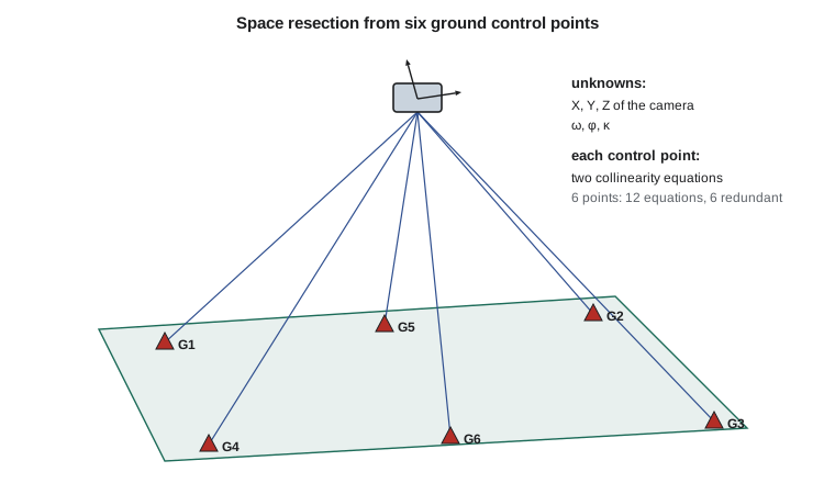
The program below carries out a resection of one corridor photo from six control points, with image measurements simulated to a precision of 3 µm, slightly better than one pixel. It starts from the centroid of the control, a level photo and a flying height 100 m too low.
# Space resection: exterior orientation of one photo from six ground control points
# by iterated least squares (Gauss-Newton with numerical partial derivatives)
import random
import math

def rot(om, ph, ka):
    """Photogrammetric rotation matrix M = R3(kappa) R2(phi) R1(omega), angles in degrees."""
    o, p, k = (math.radians(a) for a in (om, ph, ka))
    so, co, sp, cp, sk, ck = math.sin(o), math.cos(o), math.sin(p), math.cos(p), math.sin(k), math.cos(k)
    return [[cp * ck, co * sk + so * sp * ck, so * sk - co * sp * ck],
            [-cp * sk, co * ck - so * sp * sk, so * ck + co * sp * sk],
            [sp, -so * cp, co * cp]]

def project(eo, P, f):
    """Collinearity: ground point P = (X, Y, Z) -> image (x, y), same units as f."""
    XL, YL, ZL, om, ph, ka = eo
    M = rot(om, ph, ka)
    d = (P[0] - XL, P[1] - YL, P[2] - ZL)
    u, v, w = (sum(M[i][j] * d[j] for j in range(3)) for i in range(3))
    return -f * u / w, -f * v / w
def T(A): return [list(r) for r in zip(*A)]
def mul(A, B): return [[sum(a * b for a, b in zip(r, c)) for c in zip(*B)] for r in A]
def inv(A):
    n = len(A); M = [list(map(float, r)) + [1.0 if i == j else 0.0 for j in range(n)] for i, r in enumerate(A)]
    for c in range(n):
        p = max(range(c, n), key=lambda r: abs(M[r][c])); M[c], M[p] = M[p], M[c]
        d = M[c][c]; M[c] = [x / d for x in M[c]]
        for r in range(n):
            if r != c:
                f = M[r][c]; M[r] = [x - f * y for x, y in zip(M[r], M[c])]
    return [r[n:] for r in M]
def diag(v): return [[v[i] if i == j else 0.0 for j in range(len(v))] for i in range(len(v))]
def col(v): return [[x] for x in v]
random.seed(5)

ZREF = 1010.0
f = 0.100                                                     # m
truth = (10520.000, 20310.000, ZREF + 2000.0, 1.20, -0.80, 2.50)
gcp = {"G1": (9690.0, 19640.0, ZREF + 55.2), "G2": (11360.0, 19700.0, ZREF + 8.1),
       "G3": (11410.0, 20930.0, ZREF - 21.7), "G4": (9640.0, 20980.0, ZREF + 30.4),
       "G5": (10530.0, 19650.0, ZREF + 12.9), "G6": (10480.0, 20960.0, ZREF - 6.3)}
sig = 3.0e-6                                                  # image measurement precision: 3 microns
obs = {k: tuple(c + random.gauss(0, sig) for c in project(truth, P, f)) for k, P in gcp.items()}

def residuals(eo):
    v = []
    for k, P in gcp.items():
        x, y = project(eo, P, f)
        v += [obs[k][0] - x, obs[k][1] - y]
    return v

# Approximate values: middle of the control, a nominal flying height, a level photo
eo = [sum(P[0] for P in gcp.values()) / 6, sum(P[1] for P in gcp.values()) / 6, ZREF + 1900.0, 0.0, 0.0, 0.0]
steps = [0.01, 0.01, 0.01, 1e-5, 1e-5, 1e-5]
for it in range(1, 8):
    w = residuals(eo)
    A = [[0.0] * 6 for _ in w]
    for j in range(6):
        e2 = list(eo); e2[j] += steps[j]
        x2 = residuals(e2)
        for i in range(len(w)):
            A[i][j] = (w[i] - x2[i]) / steps[j]          # d(model)/d(parameter)
    N = mul(T(A), A); Q = inv(N)
    dx = [r[0] for r in mul(Q, mul(T(A), col(w)))]
    eo = [a + d for a, d in zip(eo, dx)]
    print(f"iteration {it}: |dX,dY,dZ| = {sum(d * d for d in dx[:3]) ** 0.5:10.3f} m"
          f"   max angle change {max(abs(d) for d in dx[3:]):.5f} deg")
    if max(abs(d) for d in dx[:3]) < 1e-4:
        break

v = residuals(eo)
s0 = (sum(r * r for r in v) / (len(v) - 6)) ** 0.5
print(f"Residual standard deviation {1e6 * s0:.2f} microns  (redundancy {len(v) - 6})")
names = ["XL", "YL", "ZL", "omega", "phi", "kappa"]
units = ["m", "m", "m", "deg", "deg", "deg"]
for j in range(6):
    sd = s0 * Q[j][j] ** 0.5
    fmt = "{:12.3f}" if j < 3 else "{:12.5f}"
print(f"{names[j]:6s} {fmt.format(eo[j])} {units[j]:3s} +/- {sd:.3f} {units[j]} error {eo[j] - truth[j]:+.4f}")iteration 1: |dX,dY,dZ| = 95.955 m max angle change 2.36779 deg iteration 2: |dX,dY,dZ| = 7.006 m max angle change 0.13401 deg iteration 3: |dX,dY,dZ| = 0.036 m max angle change 0.00052 deg iteration 4: |dX,dY,dZ| = 0.000 m max angle change 0.00000 deg Residual standard deviation 2.36 microns (redundancy 6) XL 10519.764 m +/- 0.151 m error -0.2365 YL 20309.736 m +/- 0.185 m error -0.2635 ZL 3009.961 m +/- 0.040 m error -0.0386 omega 1.20850 deg +/- 0.005 deg error +0.0085 phi -0.80537 deg +/- 0.004 deg error -0.0054 kappa 2.50224 deg +/- 0.001 deg error +0.0022
The first iteration corrects the position by almost 100 m and the angles by more than 2°; by the fourth the corrections are below a millimeter. The residual standard deviation, about 2.4 µm with six degrees of freedom, agrees with the simulated measurement noise. The standard deviations are revealing. The camera height is determined to about 4 cm, but the horizontal position only to about 15 to 19 cm, four times worse, and the errors of \(X_L\) and \(\varphi\), and of \(Y_L\) and \(\omega\), are large and of related size.
Correlation between position and tilt
The reason is geometric. For a nearly vertical photo, moving the camera 0.24 m west and tilting it so that its axis still points at the same ground area changes the image coordinates of every control point by almost the same small amount. A shift of \(\Delta X_L\) moves the images of all points by about \(f \Delta X_L / H\); a rotation \(\Delta \varphi\) moves them by about \(f \Delta \varphi\). The two effects nearly cancel when \(\Delta X_L \approx -H \Delta\varphi\). Only the differences between near and far points, which depend on the spread of the control in height and across the photo, can separate them. With 2000 m flying height and a 900 m wide spread of control, the separation is weak.
This correlation is harmless for the main product, because a camera position error that is compensated by a tilt error produces almost the same rays, and the ground points computed from them are almost unaffected. It matters when exterior orientation is compared with independent data, such as the navigation solution, or used for something else, such as checking the boresight calibration. A photo with control at a range of heights, such as on both the coulee rim and its floor, is better determined than one over flat ground.
Direct georeferencing
Large aerial cameras are flown with a GNSS receiver and an inertial measurement unit (IMU) tightly integrated in a navigation system, as described in GEOM-300. The GNSS antenna on the aircraft roof gives position; the IMU, mounted rigidly on the camera, gives attitude at hundreds of samples per second; and a post-processed solution, using GNSS base stations or precise point positioning and smoothing forward and backward in time, gives the trajectory of the IMU to a few centimeters and its attitude to a few thousandths of a degree. The camera sends an event pulse at the center of each exposure, and the trajectory is interpolated to that instant. The exterior orientation of every photo is then known without any ground control. This is direct georeferencing.
Two small calibrations connect the navigation solution to the camera. The lever arm is the vector from the IMU center, or from the GNSS antenna phase center, to the camera's perspective center, measured in the body frame of the aircraft. It is a few tenths of a meter to a meter or more, and it must be rotated into ground axes with the current attitude before it is added to the trajectory position. The boresight misalignment is the small rotation between the IMU axes and the camera axes, typically a few hundredths of a degree after careful mounting. It cannot be measured with a tape; it is determined by flying a calibration block over control and comparing the attitude from the IMU with the attitude from aerial triangulation.
where \(\mathbf{r}_{\text{IMU}}(t)\) is the trajectory position at the exposure time \(t\), \(\mathbf{R}_b^{\,g}\) the rotation from the body frame to ground axes, \(\mathbf{l}^{\,b}\) the lever arm in the body frame and \(\Delta\mathbf{M}_{\text{bore}}\) the boresight rotation. Any error in the attitude or in the boresight becomes a ground error proportional to the flying height.
Worked problem
Effect of an attitude error
A corridor photo is flown 2000 m above the ground with a 10 cm GSD. The boresight angle about the flight direction is in error by 0.010°. Find the resulting ground error near the nadir in meters and pixels. What attitude accuracy keeps the error below one third of a pixel?
Show solution
- \[\Delta = H \tan(0.010^\circ) = 2000 \times 1.745 \times 10^{-4} = 0.349 \text{ m}\]
- \[0.349 / 0.10 = 3.5 \text{ pixels}\]
- \[\Delta_{\max} = 0.033 \text{ m} \;\Rightarrow\; \delta = \arctan(0.033 / 2000) = 0.00095^\circ \approx 0.001^\circ\]
Answer: A boresight error of one hundredth of a degree shifts the ground by 35 cm, more than three pixels. Keeping attitude errors below a third of a pixel at this height needs an accuracy of about 0.001°, which is at the limit of high-end navigation systems and is why direct georeferencing alone rarely meets survey-grade specifications for crewed aircraft.
Integrated sensor orientation
Direct georeferencing has three weaknesses. Errors in the trajectory, boresight or interior orientation are not checked by anything, because there is no redundancy. Heights from intersecting rays are sensitive to errors in the focal length, which the navigation system cannot detect. And the trajectory can contain short-lived errors when the GNSS solution is weak, for example during sharp turns. The usual remedy is integrated sensor orientation, in which the GNSS positions and IMU attitudes enter the aerial triangulation as weighted observations together with tie points and a modest amount of ground control. The adjustment then estimates the boresight, any GNSS offsets and drifts, and the camera calibration, and the control and checkpoints verify the result. The canal project used this approach, with GNSS and IMU data for every photo and the twenty-four targets as control and checkpoints.
| Approach | Ground control needed | Strength | Weakness |
|---|---|---|---|
| Space resection, photo by photo | At least 3 per photo, preferably 6 | Simple and independent | Impractical for many photos |
| Aerial triangulation with control | A few per block, at the edges | Redundant, self-checking | Ground survey cost |
| Direct georeferencing | None (checkpoints only) | Fast, works where control is impossible | No internal check; sensitive to calibration |
| Integrated sensor orientation | Very few | Redundant and economical | Needs careful weighting and calibration |
Reference frames and heights
A GNSS trajectory is computed in the reference frame of the base stations or the precise orbit products, and its heights are ellipsoidal heights. The canal's control is in NAD83(2011) with orthometric heights in NAVD 88, as set out in GEOM-230 and GEOM-300. Before the trajectory and the ground control are combined, the trajectory must be in the same frame and epoch as the control, and the photogrammetric computation must either work in ellipsoidal heights throughout, converting to NAVD 88 afterward with the hybrid geoid model, or convert the trajectory heights first. In the Great Falls area the geoid height is about −15 m, so mixing the two height systems puts every exterior orientation 15 m too high or too low, a blunder that shows immediately as a large vertical residual on every checkpoint but can be baffling if no checkpoints were surveyed. When the NSRS modernization replaces NAVD 88 with the new geopotential datum, the same discipline applies with new models.
A further subtlety is the map projection. Collinearity is a three-dimensional relation that holds in a Cartesian system. Map projection coordinates are not Cartesian: their scale varies across the projection, and their heights refer to a curved surface. For a small area this is negligible; for a long corridor or a high flight it is not, and software either works in a local Cartesian frame and converts afterward or applies the Earth curvature correction of Lesson 3 and accepts small residual errors from projection scale. The choice should be stated in the processing report.
Checking an orientation
Whatever the method, an orientation is accepted only after it has been checked. The basic checks are the reference standard deviation against the expected image precision; the residuals at each control point, which should be small and show no pattern; the agreement between the navigation solution and the adjusted orientation, where both exist; and, most important, the differences at independent checkpoints that were not used in the solution. A resection with exactly three control points has no redundancy and cannot be checked at all; an orientation that fits its control perfectly but misses its checkpoints is wrong.
Common mistakes
MistakeClustering control points in one part of the photo.
InsteadSpread control over the whole photo and, where possible, over a range of elevations.
MistakeInterpreting the large XL and φ standard deviations as poor accuracy of the ground points.
InsteadPosition and tilt errors compensate; check the effect on ground points at checkpoints.
MistakeAdding the lever arm in ground axes without rotating it.
InsteadRotate the body-frame lever arm by the current attitude before adding it to the trajectory.
MistakeCombining ellipsoidal trajectory heights with orthometric control.
InsteadConvert with the geoid model, or work in ellipsoidal heights throughout and convert at the end.
MistakeRelying on direct georeferencing without checkpoints.
InsteadCalibrate the boresight over control and verify every project with independent checkpoints.
Summary and key terms
- Exterior orientation is found by space resection, aerial triangulation or direct georeferencing.
- Space resection solves six unknowns from at least three control points by iterated least squares.
- For near-vertical photos, horizontal position and tilt are strongly correlated; ground points are affected much less.
- Direct georeferencing measures position and attitude with GNSS and an IMU, connected to the camera by the lever arm and boresight.
- Attitude errors produce ground errors proportional to flying height; 0.01° at 2000 m is 35 cm.
- Integrated sensor orientation combines navigation data, tie points and modest control in one adjustment.
- Trajectory and control must share frame, epoch and height system before they are combined.
- Space resection
- Determination of the exterior orientation of one photo from ground control points visible in it.
- Direct georeferencing
- Determination of exterior orientation from GNSS and inertial measurements without ground control.
- Lever arm
- The vector from the IMU or GNSS antenna to the camera perspective center in the body frame.
- Boresight misalignment
- The small rotation between the IMU axes and the camera axes.
- Integrated sensor orientation
- An aerial triangulation that includes GNSS and IMU observations as weighted data.
- Reference standard deviation
- The estimated standard deviation of an observation of unit weight after adjustment.
Practice problems
Work each problem on paper first, then reveal the answer to check.
How many degrees of freedom does a resection with five control points have?
Show answer
10 observations − 6 unknowns = 4.
A lever arm of 0.80 m points forward along the aircraft's x axis and the heading is 90°. Which ground component does it affect?
Show answer
It points east, so it affects X (east) by 0.80 m.
At 100 m flying height, what ground error does a 0.05° boresight error cause?
Show answer
100 × tan(0.05°) = 0.087 m.
Why can direct georeferencing not detect an error in the focal length?
Show answer
Without redundant ground observations, a focal length error simply scales every ray and is absorbed into heights.
Why should resection control include points on both the coulee rim and floor?
Show answer
Height differences help separate camera position from tilt.
Lesson quiz · 5 questions
Score 60% or more to complete this lesson.
Create a free account to save your progress, take quizzes and earn a certificate.