
GEOM-310 · Lesson 10 of 12 · 24 min
Orthophotos
The land agents negotiating the canal easements with forty landowners wanted one thing above all: a picture of the corridor in which every fence, field approach and shelterbelt was where it really was, so that the proposed boundary could be drawn on it and measured. A raw air photo would not do, because relief displacement put the coulee rim tens of meters out of place near the edges and the grain elevators leaned like falling trees. What they needed was an orthophoto, an image with the geometry of a map. This lesson covers how orthophotos are made by differential rectification, the surface model they need, resampling, the special problems of bridges and buildings and the true orthophoto, mosaicking and radiometric balancing, the accuracy of the result and the orthophoto programs that cover the region.
From photo to orthophoto
A photograph is a central projection: every point is imaged along a ray through the perspective center, so its position depends on its height. An orthophoto is an orthogonal projection: every point is shown directly above its true horizontal position, as on a map, regardless of its height. The conversion removes three effects: tilt of the camera, the variation of scale with flying height, and relief displacement. For perfectly flat ground the first two could be removed by a projective transformation of the whole photo, a process called rectification, which was done optically in the past. Real terrain needs differential rectification, in which every small area of the image is corrected according to its own elevation.
An orthophoto combines the strengths of an image and a map. It has uniform scale, so distances and areas can be measured on it; it can be overlaid with vector data such as property boundaries, utilities and design alignments; and it shows everything the camera saw, not just the features someone chose to map. For many users, such as land agents, municipal planners and farmers, the orthophoto is the map.
Differential rectification
Modern orthophotos are produced by the indirect method, working backward from the output. The orthophoto is defined as a grid of cells in ground coordinates, for example 10 cm cells in the project grid. For each cell center \((X, Y)\), the elevation \(Z\) is interpolated from the surface model; the ground point \((X, Y, Z)\) is projected into the photo with the collinearity equations, using the exterior and interior orientation from the aerial triangulation, including lens distortion; the image coordinates are converted to a pixel position; and the brightness at that position is interpolated from the surrounding pixels and written to the orthophoto cell. Every cell is filled exactly once, and the result has no gaps.
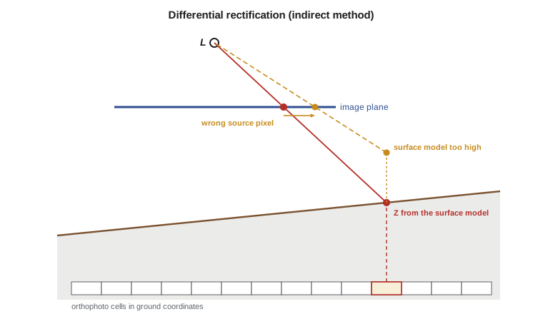
The direct method projects each image pixel to the ground by intersecting its ray with the surface model and places it in the orthophoto. It leaves gaps where the terrain stretches the image and overlaps where it compresses it, and needs extra steps to fill them, so it is rarely used for production. It is, however, the natural way to think about monoplotting from Lesson 4, and it is how a viewer of a single photo can click on a point and see its ground coordinates.
Resampling
The projected position of a cell center almost never falls exactly on a pixel center, so the brightness must be resampled. Nearest-neighbor resampling takes the value of the closest pixel; it preserves the original values, which matters for image classification, but produces jagged edges and shifts of up to half a pixel. Bilinear interpolation takes a distance-weighted average of the four surrounding pixels, giving a smoother image with slight loss of sharpness. Cubic convolution uses sixteen surrounding pixels with weights from a cubic function and keeps more sharpness at the cost of slight overshoot at strong edges. Most orthophoto production uses bilinear or cubic resampling.
where \(g_{ij}\) are the four neighboring pixel values and \(\Delta c\), \(\Delta r\) the fractional column and row offsets of the projected position from the first pixel.
The program below follows one 10 cm orthophoto cell through the whole process: elevation from a small piece of the surface model, projection into the corridor photo of Lesson 4, conversion to a pixel position, and resampling from a 3 by 3 block of brightness values. It then asks what happens if the surface model is 2 m too high at that cell.
# Differential rectification of one orthophoto cell: ground (X, Y) + DEM height -> image
# position by collinearity -> pixel -> bilinear resampling; then the cost of a DEM error
import math

def rot(om, ph, ka):
    """Photogrammetric rotation matrix M = R3(kappa) R2(phi) R1(omega), angles in degrees."""
    o, p, k = (math.radians(a) for a in (om, ph, ka))
    so, co, sp, cp, sk, ck = math.sin(o), math.cos(o), math.sin(p), math.cos(p), math.sin(k), math.cos(k)
    return [[cp * ck, co * sk + so * sp * ck, so * sk - co * sp * ck],
            [-cp * sk, co * ck - so * sp * sk, so * ck + co * sp * sk],
            [sp, -so * cp, co * cp]]

def project(eo, P, f):
    """Collinearity: ground point P = (X, Y, Z) -> image (x, y), same units as f."""
    XL, YL, ZL, om, ph, ka = eo
    M = rot(om, ph, ka)
    d = (P[0] - XL, P[1] - YL, P[2] - ZL)
    u, v, w = (sum(M[i][j] * d[j] for j in range(3)) for i in range(3))
    return -f * u / w, -f * v / w

ZREF = 1010.0
f = 0.100; pix = 5.0e-6; cols, rows = 20000, 13000
eo = (10520.000, 20310.000, ZREF + 2000.0, 1.20, -0.80, 2.50)

def dem(X, Y):                       # a small piece of the DEM: a gentle slope to the coulee
    return ZREF + 12.0 - 0.035 * (X - 10900.0) - 0.020 * (Y - 20600.0)

def to_pixel(x, y):                  # image coordinates (m, y up) -> column and row (middle of pixel 0 at 0.5)
    return x / pix + cols / 2 - 0.5, rows / 2 - y / pix - 0.5

# A 3 x 3 block of brightness values around the target pixel (columns 18058..18060, rows 3509..3511)
patch = {(18058, 3509): 118, (18059, 3509): 121, (18060, 3509): 127,
         (18058, 3510): 115, (18059, 3510): 124, (18060, 3510): 133,
         (18058, 3511): 112, (18059, 3511): 122, (18060, 3511): 138}
def bilinear(c, r):
    c0, r0 = int(c), int(r); dc, dr = c - c0, r - r0
    g = lambda i, j: patch[(c0 + i, r0 + j)]
    return (g(0, 0) * (1 - dc) * (1 - dr) + g(1, 0) * dc * (1 - dr)
            + g(0, 1) * (1 - dc) * dr + g(1, 1) * dc * dr)

X, Y = 11350.00, 20690.00            # middle of one 10 cm orthophoto cell
Z = dem(X, Y)
x, y = project(eo, (X, Y, Z), f)
c, r = to_pixel(x, y)
print(f"Ortho cell X = {X:.2f}  Y = {Y:.2f}  DEM Z = {Z:.3f}")
print(f"Image point x = {1000 * x:.4f} mm  y = {1000 * y:.4f} mm  ->  column {c:.2f}  row {r:.2f}")
print(f"Nearest-pixel value {patch[(round(c), round(r))]}, bilinear {bilinear(c, r):.1f}")

# A DEM that is 2 m too high at this cell: where does the pixel come from instead?
c2, r2 = to_pixel(*project(eo, (X, Y, Z + 2.0), f))
shift = ((c2 - c) ** 2 + (r2 - r) ** 2) ** 0.5
print(f"With the DEM 2 m too high the source pixel moves {shift:.2f} pixels = {shift * 0.10:.3f} m on the ground")
rad = 1000 * (x * x + y * y) ** 0.5
print(f"Rule of thumb dXY = dZ * r / f = 2.0 * {rad:.2f} / 100 = {2.0 * rad / 100:.3f} m")
for name, r_mm in (("principal point", 0.0), ("edge of format", 50.0), ("corner of format", 59.6)):
print(f" {name:17s} r = {r_mm:5.1f} mm displacement per m of DEM error {r_mm / 100:.3f} m")Ortho cell X = 11350.00 Y = 20690.00 DEM Z = 1004.450 Image point x = 40.2966 mm y = 14.9481 mm -> column 18058.82 row 3509.87 Nearest-pixel value 124, bilinear 122.1 With the DEM 2 m too high the source pixel moves 8.92 pixels = 0.892 m on the ground Rule of thumb dXY = dZ * r / f = 2.0 * 42.98 / 100 = 0.860 m principal point r = 0.0 mm displacement per m of DEM error 0.000 m edge of format r = 50.0 mm displacement per m of DEM error 0.500 m corner of format r = 59.6 mm displacement per m of DEM error 0.596 m
The cell at X = 11 350.00, Y = 20 690.00 takes an elevation of 1004.450 m from the surface model and projects to column 18 058.82, row 3509.87, about 43 mm from the principal point. Nearest-pixel resampling takes the value 124; bilinear interpolation gives 122.1. With the surface model 2 m too high, the source pixel moves by almost 9 pixels, so the orthophoto cell shows the ground from about 0.9 m away. The simple rule \(\Delta_{XY} = \Delta Z \cdot r/f\) predicts 0.86 m; the small difference comes from the tilt and the change in flying height above the raised surface.
The surface model and its errors
The orthophoto is only as accurate as the surface model used to make it. An elevation error \(\Delta Z\) displaces the image content horizontally by about \(\Delta Z \cdot r / f\), where \(r\) is the radial distance of the point in the photo. At the principal point the effect vanishes; at the edge of the corridor camera's format, 50 mm from the center, it is half the elevation error; at the corners, 60 mm away, it is 0.6 times. A surface model accurate to 0.2 m therefore limits the orthophoto to about 0.1 m horizontal error near the edges of each photo, a full pixel at 10 cm GSD. The usual remedies are to use only the central parts of the photos in the mosaic, which high overlap makes possible, and to use a good DTM.
Worked problem
Surface model accuracy for an orthophoto
An orthophoto with 10 cm GSD must have horizontal displacement from elevation errors below 5 cm everywhere it is used. The camera has \(f = 100\) mm, and the mosaic uses each photo only within 35 mm of its principal point. What vertical accuracy is needed in the surface model? What if the full format to the corners at 59.6 mm were used?
Show solution
- \[\Delta_{XY} = \Delta Z\,\frac{r}{f} \;\Rightarrow\; \Delta Z = \Delta_{XY}\,\frac{f}{r}\]
- \[r = 35 \text{ mm}: \quad \Delta Z = 0.05 \times \frac{100}{35} = 0.143 \text{ m}\]
- \[r = 59.6 \text{ mm}: \quad \Delta Z = 0.05 \times \frac{100}{59.6} = 0.084 \text{ m}\]
Answer: Using only the central part of each photo relaxes the surface model requirement from about 8 cm to about 14 cm. This is one of the reasons orthophoto projects are flown with more overlap than stereo mapping alone would need.
Bridges, buildings and true orthophotos
A standard orthophoto is made with a bare-earth DTM. Objects that are not part of the terrain, such as buildings, trees and bridges, are therefore not corrected: their tops are displaced by relief displacement just as in the photo, and they appear to lean away from the photo center. A building's roof is shifted off its footprint, and the side wall facing away from the center is visible. Bridges are a classic problem. The DTM follows the ground under the bridge, often the bottom of a coulee or river valley, while the bridge deck may be 20 m higher. The deck is projected using the valley floor elevation and appears bent, broken or wavy where it crosses the valley. The bridge over the coulee at the canal's second crossing looked like a ribbon draped into the valley until Theo added the deck to the surface model as a break-line-enforced surface.
A true orthophoto removes the lean of buildings and other objects by using a DSM that includes them. Every roof is then shown in its true position over its footprint. But the ground behind each building, hidden from the camera by the building, now has nothing to show: a true orthophoto must detect these occluded areas and fill them from other photos in which they are visible, which requires high overlap, both forward and side, and careful visibility analysis. True orthophotos are standard for dense urban areas where building lean would hide streets, and they are produced from the same DSM matching described in Lesson 9.
| Product | Surface used | Buildings and trees | Typical use |
|---|---|---|---|
| Rectified photo | A single plane | Displaced; terrain also displaced | Flat sites only |
| Standard orthophoto | Bare-earth DTM | Lean away from photo centers | Rural mapping, land agreements |
| Orthophoto with bridge surfaces | DTM plus bridge decks and similar | Lean, but bridges straight | Corridors and road mapping |
| True orthophoto | DSM with buildings | Upright; occluded ground filled from other photos | Dense urban areas |
Mosaicking and seamlines
An orthophoto of a project area is a mosaic of many orthorectified photos. Wherever photos overlap, a seamline divides the area taken from one from the area taken from the next. Seamlines are placed where the surface model is most reliable and where a mismatch would be least visible: along roads, field boundaries and natural features, around rather than through buildings, and through the central parts of the photos where relief displacement is smallest. Automatic seamline generation follows paths of least difference between the overlapping images, and operators edit the result where it cuts through a building or a vehicle. Mismatches along seamlines, where a road or fence line jumps sideways, are a direct measure of the relative accuracy of the orientations and the surface model; specifications often limit them to a small multiple of the GSD or of the horizontal accuracy class.
Radiometric balancing
Adjacent photos differ in brightness and color because of changes in sun angle, haze, exposure settings, and the bidirectional reflectance of the surface: fields look brighter when viewed with the sun behind the camera and darker when viewed toward the sun, and the brightest spot in each photo, the hotspot, is where the camera looks directly away from the sun. Radiometric processing corrects vignetting from the lens, balances brightness and color between photos, and blends across seamlines so that the mosaic looks like a single image. For visual use this is mostly cosmetic. For analysis, such as classifying land cover along the corridor, it changes the data, and analysts may prefer imagery with documented, physically based corrections rather than visually balanced color.
Accuracy and delivery
The horizontal accuracy of an orthophoto combines the errors of the aerial triangulation, the surface model, and the resampling. It is tested by comparing the positions of well-defined features, such as painted targets, corners of concrete pads and intersections of road markings, with their surveyed coordinates, as Lesson 12 explains. Orthophotos are delivered as georeferenced images, commonly as tiled GeoTIFF or cloud-optimized GeoTIFF files with internal overviews, together with metadata describing the coordinate system, GSD, acquisition dates, surface model, accuracy and seamlines. A tile index and a seamline layer let users find the source photo and date for any part of the mosaic, which matters when a landowner asks when a fence was built.
Orthophotos of the region come from several programs. The USDA's National Agriculture Imagery Program (NAIP) acquires four-band orthophotos of the agricultural lands of the continental United States during the growing season on a recurring cycle, now typically at about 60 cm resolution; states, counties and cities commission higher-resolution imagery; and the USGS and National Archives hold the historical photographs from which old orthophotos can be made, as Theo did for the 1962 alignment. Project orthophotos at 10 cm or better, like the canal corridor, are commissioned for their own purpose and tested against their own specification.
Common mistakes
MistakeUsing a raw air photo for measuring boundaries.
InsteadUse an orthophoto; raw photos contain tilt, scale variation and relief displacement.
MistakeMaking an orthophoto with a coarse or inaccurate DTM.
InsteadUse a DTM whose errors times r / f are within the horizontal tolerance, and the central parts of photos.
MistakeIgnoring bridges in a corridor orthophoto.
InsteadAdd bridge decks and similar elevated structures to the surface used for rectification.
MistakeCalling a DSM-based orthophoto a true orthophoto without filling occlusions.
InsteadA true orthophoto must detect occluded ground and fill it from other photos.
MistakePlacing seamlines through buildings.
InsteadRoute seamlines along roads and field edges, around buildings and through photo centers.
Summary and key terms
- An orthophoto is an image in orthogonal projection with uniform scale, made by differential rectification.
- The indirect method projects each ground cell into the photo and resamples the brightness.
- Resampling is by nearest neighbor, bilinear interpolation or cubic convolution.
- A surface model error ΔZ displaces image content by about ΔZ · r / f.
- Standard orthophotos use a DTM, so buildings lean and bridges bend; true orthophotos use a DSM and fill occlusions.
- Mosaics are joined along seamlines placed on reliable ground and balanced radiometrically.
- Orthophotos are delivered as tiled georeferenced images with metadata and seamline layers.
- Orthophoto
- An image corrected to orthogonal projection so that every point is in its true horizontal position.
- Differential rectification
- The correction of an image cell by cell according to the elevation of each cell.
- Resampling
- Interpolating brightness values at non-integer pixel positions.
- True orthophoto
- An orthophoto made with a DSM so that buildings and other objects are shown without lean.
- Seamline
- The boundary between areas taken from different photos in a mosaic.
- Hotspot
- The brightest area of a photo, where the camera looks directly away from the sun.
Practice problems
Work each problem on paper first, then reveal the answer to check.
A point is 40 mm from the principal point of a 100 mm camera, and the DTM is 0.5 m too low. How far is it displaced in the orthophoto?
Show answer
0.5 × 40 / 100 = 0.20 m along the radial direction from the photo center.
Why does nearest-neighbor resampling suit images for classification?
Show answer
It keeps the original pixel values without averaging.
A bridge deck is 18 m above the valley floor and imaged 30 mm from the principal point. How far is it displaced in a DTM-based orthophoto?
Show answer
18 × 30 / 100 = 5.4 m.
Why must true orthophotos be flown with high side overlap?
Show answer
So that ground hidden behind buildings in one photo is visible in another.
What does a sideways jump of a fence line at a seamline indicate?
Show answer
A relative error in orientation or the surface model between the two photos.
Lesson quiz · 5 questions
Score 60% or more to complete this lesson.
Create a free account to save your progress, take quizzes and earn a certificate.