
BIOL-208 · Lesson 8 of 12 · 25 min
Predation, herbivory and parasitism
Every organism is food for something else. Predators kill and eat their prey; herbivores eat plants, usually without killing them; parasites live in or on a host and draw resources from it for a long time; pathogens cause disease. All are consumer–resource interactions in which one species gains and the other loses. They are among the most powerful forces in ecology, capable of driving populations through dramatic cycles, shaping the evolution of camouflage, toxins and speed, and restructuring whole communities. This lesson develops the theory of predator–prey dynamics, the functional and numerical responses of predators, the famous ten-year cycle of snowshoe hares and lynx in the boreal forest, plant–herbivore interactions, and the ecology of parasites and wildlife disease, including chronic wasting disease in deer, elk, moose and caribou.
The Lotka–Volterra predator–prey model
Lotka and Volterra also wrote the first model of predator and prey. Prey (\( N \)) grow exponentially in the absence of predators and are killed at a rate proportional to encounters with predators (\( P \)). Predators die at a constant rate without food and produce new predators in proportion to the prey they eat:
Here \( a \) is the attack rate, \( b \) the efficiency with which eaten prey are turned into new predators, and \( m \) the predator death rate. The model predicts endless cycles: prey increase, predators increase in response, prey are eaten down, predators starve, and the cycle repeats with the predator peak lagging behind the prey peak by about a quarter of a cycle. The prey isocline is the horizontal line \( P = r/a \), and the predator isocline the vertical line \( N = m/(ba) \). The cycles are neutrally stable: their size depends entirely on the starting numbers, which is biologically unrealistic.
import numpy as np
from scipy.integrate import solve_ivp

def lv(t, y, r, a, b, m):
    N, P = y
    return [r * N - a * N * P, b * a * N * P - m * P]

sol = solve_ivp(lv, (0, 60), [40, 9], args=(0.6, 0.05, 0.4, 0.5),
                t_eval=np.arange(0, 61, 4), rtol=1e-9)
print(" t    prey  predators")
for t, N, P in zip(sol.t, *sol.y):
    print(f"{t:3.0f} {N:7.1f} {P:8.1f}")
print("prey isocline P = r/a =", 0.6 / 0.05, "; predator isocline N = m/(ba) =", 0.5 / (0.4 * 0.05))t prey predators 0 40.0 9.0 4 18.2 18.5 8 16.2 7.9 12 41.2 9.6 16 17.0 17.9 20 17.0 7.6 24 42.1 10.4 28 16.0 17.2 32 17.8 7.3 36 42.7 11.2 40 15.2 16.5 44 18.8 7.1 48 42.8 12.1 52 14.5 15.8 56 19.9 6.9 60 42.6 13.1 prey isocline P = r/a = 11.999999999999998 ; predator isocline N = m/(ba) = 24.999999999999996
Functional responses
How fast does a single predator eat prey as prey become more abundant? C. S. Holling, working at the Canadian Forest Service in Sault Ste. Marie, Ontario in the late 1950s, studied small mammals eating sawfly cocoons and described three types of functional response. In a Type I response, the kill rate rises in a straight line with prey density, up to a sharp maximum, as in filter feeders. In a Type II response, the kill rate rises but levels off, because each prey takes time to catch and eat (the handling time), so a predator cannot eat faster than one prey per handling time however abundant prey become. In a Type III response, the curve is S-shaped: predators eat few prey when prey are rare, perhaps because they hunt elsewhere or have not learned to find them, then switch to the prey as it becomes common. Holling's famous "disc equation" for Type II came from an experiment in which a blindfolded assistant picked up sandpaper discs from a table.
Here \( a \) is the attack rate and \( h \) the handling time. At high prey density, \( f(N) \) approaches \( 1/h \). The type of response matters for stability. A Type II response means the proportion of prey eaten falls as prey increase, which can destabilize populations; a Type III response means predators take a growing share of prey as prey increase, which can hold prey at low density.
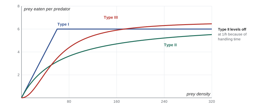
def type1(N, a=0.1, cap=6): return min(a * N, cap)
def type2(N, a=0.1, h=0.15): return a * N / (1 + a * h * N)
def type3(N, a=0.002, h=0.15): return a * N**2 / (1 + a * h * N**2)

print(" prey   Type I  Type II  Type III   (prey eaten per predator per day)")
for N in (5, 10, 20, 40, 80, 160, 320):
    print(f"{N:5d} {type1(N):8.2f} {type2(N):8.2f} {type3(N):9.2f}")
print("Type II ceiling = 1/h =", round(1 / 0.15, 2), "prey per day") prey Type I Type II Type III (prey eaten per predator per day)
5 0.50 0.47 0.05
10 1.00 0.87 0.19
20 2.00 1.54 0.71
40 4.00 2.50 2.16
80 6.00 3.64 4.38
160 6.00 4.71 5.90
320 6.00 5.52 6.46
Type II ceiling = 1/h = 6.67 prey per dayPredators also show a numerical response: their numbers rise when prey are abundant, through better reproduction and survival or by moving into prey-rich areas. Together, the functional and numerical responses determine the total predation rate. A more realistic predator–prey model, developed by Michael Rosenzweig and Robert MacArthur in 1963, combines logistic prey growth with a Type II functional response. It shows that predator–prey systems can settle to a stable equilibrium or produce cycles of a fixed size, depending on parameters. A surprising prediction, the paradox of enrichment, is that increasing the prey's carrying capacity, for example by adding nutrients, can destabilize the system into large cycles that risk extinction.
import numpy as np
from scipy.integrate import solve_ivp

def rm(t, y, r, K, a, h, b, m):
    N, P = y
    f = a * N / (1 + a * h * N)
    return [r * N * (1 - N / K) - f * P, b * f * P - m * P]

for K in (30, 200):
    sol = solve_ivp(rm, (0, 600), [30, 5], args=(1.0, K, 0.1, 0.5, 0.5, 0.3),
                    t_eval=np.linspace(400, 600, 2001), rtol=1e-8)
    N = sol.y[0]
    print(f"K = {K:3d}: prey range in the last 200 time units {N.min():6.2f} to {N.max():6.2f}"
+ (" (stable equilibrium)" if N.max() - N.min() < 1 else " (cycles)"))K = 30: prey range in the last 200 time units 8.57 to 8.57 (stable equilibrium) K = 200: prey range in the last 200 time units 0.00 to 199.31 (cycles)
The snowshoe hare cycle
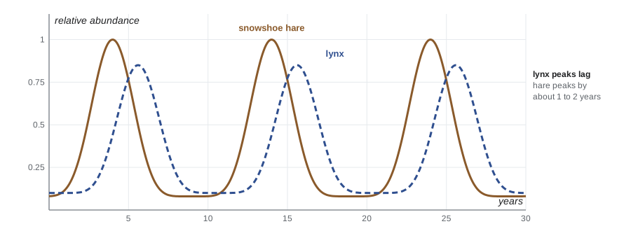
The fur-trading records of the Hudson's Bay Company, analyzed by Charles Elton in the 1920s and 1930s, revealed that lynx pelts traded from across the boreal forest rose and fell in a cycle of about ten years, following a similar cycle in snowshoe hares. Hare densities at the peak can be 10 to 25 times higher than in the low phase. For decades it was assumed the cycle was a simple predator–prey oscillation, but it is more complex. From 1986 to 1996, Charles Krebs, Stan Boutin, Rudy Boonstra and colleagues ran a large experiment near Kluane Lake in the southwestern Yukon. On 1 km² blocks of forest, they added food, excluded mammalian predators with electric fences, or did both. Adding food alone raised hare density about threefold but did not stop the cycle; excluding predators doubled density; doing both raised density about elevenfold. The conclusion was that the cycle arises from the interaction of predation and food, with predation the dominant factor. Later work by Boonstra showed that the fear of predators also matters: stressed hares in the decline phase produce fewer and smaller young, which helps explain why the low phase lasts for years after predators decline.
Prey defenses
Predation is a strong selective force, and prey have evolved many defenses. Some avoid detection through camouflage, as the snowshoe hare's coat changes from brown in summer to white in winter. Some are protected chemically: monarch butterflies store toxic cardiac glycosides from milkweed and advertise them with bright warning colors (aposematism). Harmless species may mimic toxic ones (Batesian mimicry), while several toxic species may share a warning pattern (Müllerian mimicry); the viceroy butterfly, once considered a Batesian mimic of the monarch, turned out to be distasteful itself. Other defenses include armor, spines, speed, vigilance and grouping: musk oxen form a defensive ring around their calves when wolves approach. As climate change shortens the snow season, white hares on brown ground are increasingly exposed, an example of camouflage mismatch now documented in North America.
Herbivory
Herbivores rarely kill the plants they eat, but they can reduce growth, reproduction and survival, and they shape which plants dominate. Plants defend themselves with physical structures such as thorns, tough leaves and silica, and with chemicals such as tannins, alkaloids and terpenes. Some defenses are always present (constitutive); others are induced only after attack. Birch and aspen in the boreal forest produce resinous, less palatable twigs after heavy browsing by hares, which may contribute to the hare cycle. Plants also tolerate herbivory by regrowing quickly from protected buds, as grasses do from the base. Herbivore outbreaks can transform forests: the spruce budworm, a native moth, defoliates balsam fir and spruce across millions of hectares of eastern Canada and Maine in outbreaks every 30 to 40 years.
Parasites and pathogens
Parasites live in or on a host and harm it without usually killing it quickly. Microparasites such as viruses, bacteria and protozoa multiply inside the host and are usually studied as infections spreading through a population. Macroparasites such as worms, ticks and lice are visible and are counted individually. Many parasites have complex life cycles involving several hosts: the meningeal worm of white-tailed deer, harmless to deer, is fatal to moose and caribou that eat infected snails, which may limit moose where deer are abundant. Winter ticks can carry tens of thousands of individuals on a single moose, causing hair loss and calf deaths in New England, Quebec and the Prairies, a problem that has worsened with shorter winters.
Epidemiologists model infectious disease by dividing the host population into compartments: susceptible (S), infected (I) and recovered or removed (R). In the simplest SIR model, the basic reproduction number \( R_0 \) is the average number of new infections caused by one infected individual in a fully susceptible population. An outbreak grows only if \( R_0 > 1 \). For wildlife, a key question is whether transmission depends on host density (more contacts in crowded populations) or on the frequency of infected individuals (as for sexually transmitted diseases), because density-dependent diseases die out when hosts become rare, while frequency-dependent ones can drive hosts to extinction.
import numpy as np
from scipy.integrate import solve_ivp

def sir(t, y, beta, gamma):
    S, I, R = y
    return [-beta * S * I, beta * S * I - gamma * I, gamma * I]

N0 = 1000
for beta in (0.0002, 0.0006):
    gamma = 0.25
    R0 = beta * N0 / gamma
    sol = solve_ivp(sir, (0, 200), [N0 - 1, 1, 0], args=(beta, gamma), dense_output=True, rtol=1e-8)
    t = np.linspace(0, 200, 2001); S, I, R = sol.sol(t)
    print(f"beta = {beta}: R0 = {R0:.2f}, peak infected {I.max():6.1f} at day {t[I.argmax()]:5.1f}, "
f"total ever infected {R[-1] + I[-1]:6.1f}")beta = 0.0002: R0 = 0.80, peak infected 1.0 at day 0.0, total ever infected 4.9 beta = 0.0006: R0 = 2.40, peak infected 219.0 at day 20.6, total ever infected 878.8
Chronic wasting disease (CWD) is a fatal, incurable prion disease of deer, elk, moose and caribou. Misfolded prion proteins accumulate in the brain, and infected animals shed prions in saliva, urine and faeces for months before they show signs; prions can persist in soil for years. Because prevalence keeps rising slowly over decades rather than flaring and fading, CWD behaves more like a frequency-dependent disease with an environmental reservoir than a classic SIR epidemic.
In the United States, CWD has spread from a small area of Colorado and Wyoming, where it was first recognized in the 1960s and 1970s, to wild or farmed cervids in 37 states as of June 2026, according to the US Geological Survey's distribution map, which also lists five Canadian provinces. State wildlife agencies run surveillance programs that rely on hunters submitting samples, and the US Department of Agriculture regulates farmed cervids. In 2026 the US Fish and Wildlife Service updated its response strategy for the National Elk Refuge in Wyoming, where elk crowd onto winter feedgrounds. No human cases have been documented, but the Centers for Disease Control and Prevention advises against eating meat from animals that test positive.
Managing wildlife disease draws on the ecology covered in this course. Winter feeding concentrates animals and raises transmission; culling to reduce density can slow density-dependent diseases but is controversial; and movements of live animals between farms or regions have spread diseases far faster than natural dispersal. White-nose syndrome, a fungal disease that has killed millions of bats in eastern North America since 2006, and the amphibian chytrid fungus show how introduced pathogens can devastate naive hosts.
| Interaction | Effect on consumer | Effect on resource | Example |
|---|---|---|---|
| Predation | + | − (killed) | Lynx eating snowshoe hares |
| Herbivory | + | − (usually not killed) | Moose browsing balsam fir |
| Parasitism | + | − (harmed, usually not killed quickly) | Winter ticks on moose |
| Disease (pathogen) | + | − (sometimes fatal) | Chronic wasting disease in deer |
| Parasitoid | + | − (killed eventually) | Wasps laying eggs in spruce budworm larvae |
Common mistakes
MistakePredators always control their prey populations.
InsteadPredation interacts with food, disease and weather; in the hare cycle, food and predation act together.
MistakeLotka–Volterra predator–prey cycles are stable at a fixed size.
InsteadThey are neutrally stable, with size set by starting numbers; more realistic models give stable equilibria or limit cycles.
MistakeA Type II functional response means predators eat more as prey increase without limit.
InsteadKill rate levels off at 1/h because each prey takes handling time.
MistakeAdding nutrients always stabilizes a food chain.
InsteadThe paradox of enrichment shows that raising prey carrying capacity can produce large, destabilizing cycles.
MistakeAn outbreak spreads whenever there is at least one infected host.
InsteadIt grows only if R₀ exceeds 1.
Summary and key terms
- Predation, herbivory, parasitism and disease are consumer–resource interactions (+/−).
- The Lotka–Volterra predator–prey model gives neutral cycles with predator peaks lagging prey peaks.
- Holling described Type I, II and III functional responses; Type II levels off at 1/h because of handling time.
- Logistic prey and Type II predators (Rosenzweig–MacArthur) give equilibria or limit cycles; enrichment can destabilize.
- The ten-year snowshoe hare cycle results from predation and food acting together, as the Kluane experiment showed.
- Prey defend themselves by camouflage, toxins, mimicry and behavior; plants use physical, chemical and induced defenses.
- Disease spreads only if R₀ > 1; chronic wasting disease is spreading slowly across North America.
- functional response
- How a predator's kill rate changes with prey density.
- numerical response
- How predator numbers change with prey density.
- handling time
- Time a predator spends catching and eating each prey.
- paradox of enrichment
- Increasing prey carrying capacity can destabilize predator–prey dynamics.
- aposematism
- Bright colors that advertise a prey's toxicity or danger.
- Batesian mimicry
- A harmless species resembling a harmful one.
- induced defense
- A plant defense produced only after herbivore attack.
- parasitoid
- An insect whose larvae develop in or on a host and eventually kill it.
- basic reproduction number (R₀)
- The average number of new infections caused by one infected individual in a fully susceptible population.
- prion
- A misfolded protein that causes other proteins to misfold, as in chronic wasting disease.
Practice problems
Work each problem on paper first, then reveal the answer to check.
In the Lotka–Volterra model with r = 0.8 and a = 0.04, where is the prey isocline?
Show answer
P = r/a = 20 predators.
With b = 0.5, a = 0.04 and m = 0.6, where is the predator isocline?
Show answer
N = m/(ba) = 0.6/0.02 = 30 prey.
A predator has handling time 0.2 days per prey. What is its maximum kill rate?
Show answer
1/h = 5 prey per day.
Calculate the Type II kill rate at N = 50 with a = 0.1 and h = 0.2.
Show answer
0.1 × 50 / (1 + 0.1 × 0.2 × 50) = 5/2 = 2.5 prey per day.
Which functional response can stabilize prey at low density, and why?
Show answer
Type III, because predators eat a rising proportion of prey as prey increase.
What did the Kluane experiment show about the hare cycle?
Show answer
Food addition and predator exclusion together raised density about elevenfold; both factors matter, predation most.
Give one plant defense that is induced and one that is constitutive.
Show answer
Induced: resinous twigs after browsing. Constitutive: thorns or tannins always present.
In an SIR model, β = 0.0004, S₀ = 1,000 and γ = 0.2. Calculate R₀.
Show answer
0.0004 × 1,000 / 0.2 = 2.
Why is chronic wasting disease hard to eradicate?
Show answer
Prions persist in soil for years, infected animals shed them before showing signs, and there is no cure or vaccine.
Why might winter feeding of deer increase disease?
Show answer
It concentrates animals, raising contact and transmission.
Lesson quiz · 5 questions
Score 60% or more to complete this lesson.
Create a free account to save your progress, take quizzes and earn a certificate.