
BIOL-208 · Lesson 5 of 12 · 25 min
Life histories and demography
A sockeye salmon hatches in a gravel bed in a British Columbia tributary of the Fraser River, spends a year or two in a lake, two years at sea, returns to its natal stream, spawns once and dies. A black bear may live 25 years, first breed at four or five, and raise a small litter every second year. A dandelion sets thousands of seeds within weeks of germinating. These differences in the timing of growth, reproduction and death are called life histories, and they determine how fast populations can grow and how they respond to harvest, habitat loss and conservation. Lesson 4 treated all individuals in a population as identical. This lesson adds age and stage: how ecologists measure survival and reproduction at each age using life tables, how they project populations with matrix models, and how natural selection shapes life histories through trade-offs.
Life tables
A life table summarizes how survival and reproduction change with age. A cohort life table follows a group of individuals born at the same time until all have died, which is practical for short-lived organisms or long-term field studies. A static (or time-specific) life table instead records the ages of individuals alive, or at death, at one time and assumes the population is stable. The standard columns are:
| Symbol | Meaning | How it is calculated |
|---|---|---|
| x | Age class | Usually in years |
| nₓ | Number alive at the start of age x | Counted |
| lₓ | Survivorship: proportion of the original cohort alive at age x | nₓ / n₀ |
| dₓ | Number dying during age x | nₓ − nₓ₊₁ |
| qₓ | Age-specific mortality rate | dₓ / nₓ |
| mₓ (or bₓ) | Average number of female offspring per female of age x | Counted |
| lₓmₓ | Expected offspring at age x per newborn female | lₓ × mₓ |
| eₓ | Life expectancy at age x | Mean further years for individuals alive at x |
From the life table, three key numbers summarize the population. The net reproductive rate, \( R_0 \), is the average number of female offspring a newborn female produces in her lifetime. The generation time, \( T \), is the average age at which females give birth. The intrinsic rate of increase can then be approximated:
If \( R_0 > 1 \), each female more than replaces herself and the population grows; if \( R_0 < 1 \), it declines.
import numpy as np

# Invented cohort life table for a small mammal (females only)
x  = np.array([0, 1, 2, 3, 4, 5])
n  = np.array([1000, 300, 160, 70, 20, 0])
m  = np.array([0.0, 1.2, 2.6, 2.8, 2.0, 0.0])
lx = n / n[0]
dx = n - np.append(n[1:], 0)
qx = np.divide(dx, n, out=np.zeros(len(n)), where=n > 0)
lm = lx * m
R0 = lm.sum(); T = (x * lm).sum() / R0; r = np.log(R0) / T
print(" x    nx    lx     dx    qx     mx   lxmx")
for row in zip(x, n, lx, dx, qx, m, lm):
    print("{:2d} {:5d} {:6.3f} {:5d} {:6.3f} {:5.1f} {:6.3f}".format(*row))
print(f"R0 = {R0:.3f} T = {T:.2f} years r = {r:.3f} per year")x nx lx dx qx mx lxmx 0 1000 1.000 700 0.700 0.0 0.000 1 300 0.300 140 0.467 1.2 0.360 2 160 0.160 90 0.562 2.6 0.416 3 70 0.070 50 0.714 2.8 0.196 4 20 0.020 20 1.000 2.0 0.040 5 0 0.000 0 0.000 0.0 0.000 R0 = 1.012 T = 1.92 years r = 0.006 per year
In this invented population, a newborn female produces almost exactly one daughter over her life (R₀ ≈ 1.01), the average age of mothers is about 1.9 years, and the population is nearly stable, growing at well under 1 percent a year. A small drop in first-year survival would tip it into decline. Note that 70 percent of individuals die in their first year: high juvenile mortality is common in nature, and it means that what happens to the young often controls population growth.
Survivorship curves
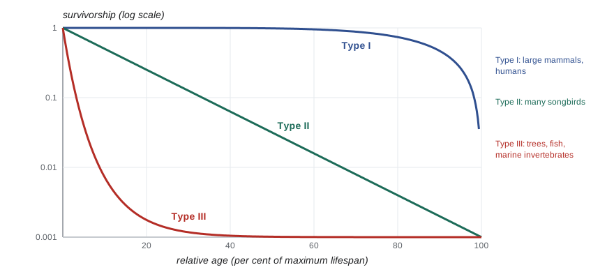
Plotting \( l_x \) on a logarithmic scale against age gives a survivorship curve. Raymond Pearl described three idealized types in 1928. Type I curves stay high until old age and then drop, as in humans in wealthy countries and many large mammals that invest heavily in few offspring. Type II curves fall in a straight line on the log scale, meaning a constant mortality rate at every age, as in many songbirds once they leave the nest. Type III curves plunge early and then flatten, as in trees, fish and marine invertebrates that produce huge numbers of tiny offspring, almost all of which die young. Real species mix these shapes, but the types are a useful shorthand.
Matrix population models
Life tables summarize the past; matrix models project the future. Patrick Leslie introduced the approach in 1945. The population is divided into age classes, and a matrix gives the fecundity of each class (top row) and the probability of surviving from one class to the next (sub-diagonal). Multiplying the matrix by the vector of numbers in each class gives the numbers one time step later:
After many time steps, the proportions in each class settle into the stable age distribution, and the population grows by a constant factor each step. That factor is the dominant eigenvalue of the matrix, which equals \( \lambda \), and the stable age distribution is its corresponding eigenvector. Matrix models extend naturally to stages rather than ages, which is often more useful: a tree's fate depends on its size, not its age, and a turtle's on whether it is an egg, a juvenile or an adult.
import numpy as np

A = np.array([[0.0, 1.5, 2.2],
              [0.4, 0.0, 0.0],
              [0.0, 0.6, 0.5]])     # last class: adults that survive and stay adults
n = np.array([100.0, 0.0, 0.0])
for t in range(1, 6):
    n = A @ n
    print(f"year {t}: " + "  ".join(f"{v:7.1f}" for v in n) + f"   total {n.sum():7.1f}")
vals, vecs = np.linalg.eig(A)
i = np.argmax(vals.real)
lam = vals[i].real
w = np.abs(vecs[:, i].real); w = w / w.sum()
print(f"dominant eigenvalue lambda = {lam:.3f}  (r = {np.log(lam):.3f})")
print("stable stage distribution:", np.round(w, 3))year 1: 0.0 40.0 0.0 total 40.0 year 2: 60.0 0.0 24.0 total 84.0 year 3: 52.8 24.0 12.0 total 88.8 year 4: 62.4 21.1 20.4 total 103.9 year 5: 76.6 25.0 22.9 total 124.4 dominant eigenvalue lambda = 1.175 (r = 0.162) stable stage distribution: [0.609 0.207 0.184]
Sensitivity and elasticity
Matrix models answer a practical question: if we could improve survival or reproduction at one stage, which would raise \( \lambda \) the most? Elasticity measures the proportional change in \( \lambda \) caused by a proportional change in one matrix element. In a famous analysis in 1987, Deborah Crouse and colleagues built a stage-based model of loggerhead sea turtles in the southeastern United States. Conservation had focused on protecting eggs and nesting beaches, but the model showed that \( \lambda \) was far more sensitive to the survival of large juveniles and subadults, which were drowning in shrimp trawls. This analysis supported the requirement for turtle excluder devices in US shrimp nets. The same logic is now used for species from orcas to orchids.
import numpy as np

A = np.array([[0.0, 1.5, 2.2],
              [0.4, 0.0, 0.0],
              [0.0, 0.6, 0.5]])
vals, W = np.linalg.eig(A); vals_l, V = np.linalg.eig(A.T)
i = np.argmax(vals.real); j = np.argmax(vals_l.real)
lam = vals[i].real
w = np.abs(W[:, i].real); v = np.abs(V[:, j].real)
S = np.outer(v, w) / (v @ w)          # sensitivities
E = S * A / lam                        # elasticities (sum to 1)
names = ["F1", "F2", "F3", "P1", "-", "-", "-", "P2", "P3"]
for (r, c), e in np.ndenumerate(E):
    if A[r, c] > 0:
        print(f"element A[{r},{c}] = {A[r, c]:.1f}   elasticity {e:.3f}")
print("sum of elasticities:", round(E.sum(), 3))element A[0,1] = 1.5 elasticity 0.145 element A[0,2] = 2.2 elasticity 0.190 element A[1,0] = 0.4 elasticity 0.335 element A[2,1] = 0.6 elasticity 0.190 element A[2,2] = 0.5 elasticity 0.140 sum of elasticities: 1.0
Life history trade-offs
Organisms have limited energy and time, so investing more in one function means investing less in another. These trade-offs shape life histories. A female can produce many small offspring or a few large ones; she can breed early and risk her own survival, or delay breeding and grow; she can breed once in a massive effort or spread reproduction over many seasons. Experiments confirm the costs: when ecologists enlarged clutches of collared flycatchers by adding eggs, parents raised more young that year but survived less well and produced fewer young later.
Breeding once and dying, as Pacific salmon, many annual plants and agave do, is called semelparity. Breeding repeatedly, as most birds, mammals and perennial plants do, is iteroparity. Semelparity is favored when adult survival between breeding attempts is low or when a huge single effort is far more productive than several small ones, as when salmon must make a costly migration to spawn. Interestingly, Atlantic salmon, unlike Pacific species, can survive to spawn again.
In the 1960s, Robert MacArthur and E. O. Wilson described a contrast between r-selected species, favored in unpredictable or newly opened habitats, which mature early and produce many small offspring, and K-selected species, favored in crowded, stable habitats, which mature late, produce few large offspring and invest heavily in each. The scheme proved too simple, and ecologists now usually describe a fast–slow continuum of life histories, with mice, annual weeds and many insects at the fast end and elephants, albatrosses, whales and bristlecone pines at the slow end. Position on the continuum predicts how a species responds to threats: slow species recover slowly from losses of adults, which is why long-lived sharks, sturgeon and rockfish are so vulnerable to overfishing.
| Trait | Fast end | Slow end |
|---|---|---|
| Age at first reproduction | Early | Late |
| Offspring per breeding event | Many | Few |
| Size of offspring | Small | Large |
| Parental care | Little | Extensive |
| Lifespan | Short | Long |
| Typical survivorship | Type III | Type I |
| Examples | House mouse, dandelion, aphid | Grizzly bear, bowhead whale, lake sturgeon |
Worked problem
Will this population persist?
A lake sturgeon population has R₀ = 0.85 and a generation time of 30 years. Estimate r and the time for the population to halve.
Show solution
- r ≈ ln R₀ / T = ln 0.85 / 30 = −0.1625 / 30 ≈ −0.0054 per year.
- Halving time = ln 2 / |r| = 0.693 / 0.0054 ≈ 128 years.
- The decline is slow but steady, and recovery would also be slow even if R₀ rose above 1.
Answer: r ≈ −0.005 per year; the population halves in about 130 years. Long-lived, late-maturing species show slow declines that are easy to miss and slow to reverse.
Common mistakes
Mistakelₓ is the proportion of individuals that die at age x.
Insteadlₓ is the proportion of the original cohort still alive at age x; qₓ is the mortality rate during age x.
MistakeR₀ is the growth rate per year.
InsteadR₀ is the average lifetime female offspring per female, measured per generation; r is per unit time.
MistakeThe stable age distribution means the population has stopped growing.
InsteadIt means the proportions in each class are constant; the population can still grow or shrink at rate λ.
MistakeProtecting eggs always helps a population the most.
InsteadElasticity analysis often shows that survival of older juveniles or adults matters more, as with loggerhead turtles.
Mistaker- and K-selection are two distinct categories.
InsteadLife histories lie on a continuum from fast to slow, and many species mix traits.
Summary and key terms
- Life tables record survival (lₓ), mortality (qₓ) and fecundity (mₓ) by age.
- R₀ = Σ lₓmₓ, T = Σ x lₓmₓ / R₀, and r ≈ ln R₀ / T.
- Survivorship curves are idealized as Type I (late mortality), II (constant) and III (early mortality).
- Leslie and stage matrices project populations; the dominant eigenvalue is λ and its eigenvector is the stable distribution.
- Elasticity analysis identifies the vital rates with the greatest effect on λ and guides conservation.
- Trade-offs shape life histories: number versus size of offspring, current versus future reproduction, semelparity versus iteroparity.
- Life histories lie on a fast–slow continuum that predicts vulnerability to harvest.
- life table
- A table of survival, mortality and fecundity by age.
- survivorship (lₓ)
- The proportion of a cohort surviving to age x.
- net reproductive rate (R₀)
- Average lifetime female offspring per female.
- generation time (T)
- The average age of mothers when their offspring are born.
- Leslie matrix
- A matrix of age-specific fecundities and survival probabilities used to project a population.
- stable age distribution
- The constant proportions in each age class reached after many time steps.
- elasticity
- The proportional change in λ caused by a proportional change in a vital rate.
- semelparity
- Reproducing once in a lifetime and then dying.
- iteroparity
- Reproducing repeatedly over a lifetime.
- trade-off
- A situation in which investing more in one trait requires investing less in another.
Practice problems
Work each problem on paper first, then reveal the answer to check.
A cohort of 500 has 200 alive at age 1. What is l₁?
Show answer
200/500 = 0.4.
If n₂ = 120 and n₃ = 90, what is q₂?
Show answer
(120 − 90)/120 = 0.25.
A life table gives lₓmₓ values of 0, 0.6, 0.5 and 0.2 at ages 0–3. Calculate R₀.
Show answer
0 + 0.6 + 0.5 + 0.2 = 1.3.
For the same table, calculate T.
Show answer
(1 × 0.6 + 2 × 0.5 + 3 × 0.2)/1.3 = 2.2/1.3 ≈ 1.69 years.
Estimate r from R₀ = 1.3 and T = 1.69.
Show answer
ln 1.3 / 1.69 ≈ 0.155 per year.
Which survivorship type fits an oak tree?
Show answer
Type III: acorns and seedlings die in vast numbers; survivors live long.
What does the dominant eigenvalue of a Leslie matrix represent?
Show answer
The asymptotic growth factor λ per time step.
Why did elasticity analysis of loggerhead turtles change policy?
Show answer
It showed survival of large juveniles mattered more than egg survival, supporting turtle excluder devices.
Why are Pacific salmon semelparous?
Show answer
The costly migration lowers survival between breeding attempts, favoring one large reproductive effort.
Why are slow life-history species vulnerable to overfishing?
Show answer
They mature late and reproduce slowly, so losses of adults are replaced only slowly.
Lesson quiz · 5 questions
Score 60% or more to complete this lesson.
Create a free account to save your progress, take quizzes and earn a certificate.