
BIOL-208 · Lesson 10 of 12 · 24 min
Succession, disturbance and island biogeography
Communities are never fixed. A forest burns and is replaced first by fireweed and aspen, then by spruce; a glacier retreats and leaves bare gravel that becomes, over two centuries, a spruce and hemlock forest; a farmer abandons a field and it fills with goldenrod, then shrubs, then trees. These directional changes in community composition after disturbance are called succession. This lesson examines how succession proceeds and why, the role of disturbance in shaping communities, how ecologists have argued about whether communities are tightly organized units or loose collections of species, and the theory of island biogeography, which explains why large, nearby islands, lakes and habitat patches hold more species than small, remote ones.
Primary and secondary succession
Primary succession begins on surfaces with no soil and no living organisms: rock exposed by a retreating glacier, fresh lava, or new sand dunes. Secondary succession begins where a disturbance has removed most organisms but left the soil, with its seeds, roots and microbes: after fire, logging, windthrow, flood or the abandonment of farmland. Secondary succession is usually much faster because soil and propagules are already present.
The classic study of primary succession is at Glacier Bay in southeastern Alaska, where glaciers have retreated about 100 km since the late eighteenth century, leaving a sequence of surfaces of known age. William Cooper began studying it in 1916. Near the ice, bare gravel is colonized by mosses, lichens, horsetails and mountain avens (Dryas), a low plant whose roots host nitrogen-fixing bacteria. Then come willows and Sitka alder, which also fix nitrogen and build up soil nitrogen and organic matter rapidly. After several decades, Sitka spruce overtops the alder, and after a century or two, western hemlock joins the spruce. Later work by F. Stuart Chapin and colleagues showed that the sequence is not simply one stage preparing the way for the next: some species facilitate later ones, but others inhibit them, and the order depends partly on which seeds arrive first.
Mount St. Helens in Washington offered a natural experiment after its eruption in 1980. Ecologists found that recovery was patchy and depended on legacies: surviving plants under snow, buried roots, gophers that churned up soil, and logs that sheltered small animals. Surfaces with biological legacies recovered far faster than sterile pumice plains, emphasizing that even large disturbances rarely start succession from zero.
Mechanisms of succession
In 1977, Joseph Connell and Ralph Slatyer proposed three models of how early species affect later ones. In the facilitation model, early colonists change conditions in ways that make the site more suitable for later species, as nitrogen-fixing alder does at Glacier Bay. In the tolerance model, later species are simply those that can tolerate lower resource levels, such as shade, and they replace earlier species by outcompeting them as resources become scarce. In the inhibition model, early species hold the site and resist invasion; later species replace them only when they die or are damaged. All three operate in nature, often in the same succession, and life-history traits help explain the order: pioneer species tend to have small, widely dispersed seeds, fast growth and high light requirements, while late-successional species have larger seeds, slower growth and greater shade tolerance.
| Trait | Early-successional (pioneer) | Late-successional |
|---|---|---|
| Seed size and number | Small and many | Large and few |
| Dispersal | Wind or birds, long distance | Animals or gravity, shorter distance |
| Growth rate | Fast | Slow |
| Shade tolerance | Low | High |
| Lifespan | Short | Long |
| Examples in eastern Canada and the northeastern US | Fireweed, trembling aspen, white birch, pin cherry | Sugar maple, American beech, eastern hemlock |
Succession can be modeled as a Markov chain, in which each spot in a forest has a probability of changing from one species to another over a time step, depending on which seedlings grow up under each canopy tree. Henry Horn used this approach for forests in New Jersey in the 1970s. Repeatedly applying the transition matrix gives the long-run composition, which does not depend on the starting point.
import numpy as np

states = ["aspen", "birch", "red maple", "sugar maple", "beech"]
# Probability that a canopy tree of each row is replaced by each column after ~50 years (illustrative)
T = np.array([
    [0.05, 0.10, 0.35, 0.30, 0.20],
    [0.02, 0.05, 0.30, 0.40, 0.23],
    [0.01, 0.03, 0.15, 0.45, 0.36],
    [0.00, 0.01, 0.07, 0.52, 0.40],
    [0.00, 0.01, 0.05, 0.34, 0.60],
])
x = np.array([1.0, 0, 0, 0, 0])   # start: pure aspen after a fire
for step in range(1, 7):
    x = x @ T
    print(f"after {step * 50:3d} years: " + "  ".join(f"{s} {p:.2f}" for s, p in zip(states, x)))
vals, vecs = np.linalg.eig(T.T)
st = np.real(vecs[:, np.argmax(np.real(vals))]); st = st / st.sum()
print("long-run composition:", " ".join(f"{s} {p:.2f}" for s, p in zip(states, st)))after 50 years: aspen 0.05 birch 0.10 red maple 0.35 sugar maple 0.30 beech 0.20 after 100 years: aspen 0.01 birch 0.03 red maple 0.13 sugar maple 0.44 beech 0.40 after 150 years: aspen 0.00 birch 0.01 red maple 0.08 sugar maple 0.43 beech 0.47 after 200 years: aspen 0.00 birch 0.01 red maple 0.07 sugar maple 0.43 beech 0.49 after 250 years: aspen 0.00 birch 0.01 red maple 0.07 sugar maple 0.43 beech 0.49 after 300 years: aspen 0.00 birch 0.01 red maple 0.07 sugar maple 0.42 beech 0.49 long-run composition: aspen 0.00 birch 0.01 red maple 0.07 sugar maple 0.42 beech 0.49
The climax debate
Early in the twentieth century, Frederic Clements argued that succession leads to a single, predictable climax community determined by climate, and that a community behaves almost like a superorganism, developing through stages as an individual does. Henry Gleason disagreed: in his individualistic concept (1926), each species responds independently to the environment, and a community is simply the set of species whose tolerances happen to overlap at a place. Whittaker's studies of vegetation along gradients in the Great Smoky Mountains and other ranges in the 1950s and 1960s supported Gleason: species replaced one another gradually and independently along gradients, without sharp boundaries between discrete communities. The pollen record, which shows species migrating separately after the last glaciation and forming combinations that do not exist today, supports the same view. Most ecologists now treat communities as loosely organized and the climax as a shifting mosaic rather than a fixed endpoint.
Disturbance regimes
A disturbance is a relatively discrete event that removes organisms and opens space or resources, such as fire, windstorm, flood, insect outbreak or grazing. Ecologists describe a disturbance regime by its type, frequency, intensity, size and season. Many ecosystems depend on recurring disturbance. The boreal forest is a fire-driven system: large, intense crown fires burn through stands of black spruce and jack pine every 50 to 200 years or so, depending on region. Jack pine and lodgepole pine have serotinous cones sealed with resin that open only in the heat of a fire, releasing seeds onto freshly burned ground; black spruce has semi-serotinous cones. Without fire, these species would be replaced.
If fires strike randomly with respect to stand age, the proportion of a landscape older than age \( t \) follows a negative exponential distribution, and the fire cycle, the time needed to burn an area equal to the whole landscape, equals the mean stand age. Ecologists estimate fire cycles from the age structure of forests and from fire scars on trees.
import numpy as np

for b in (60, 100, 200):              # fire cycle in years
    share_old = np.exp(-150 / b)
    share_young = 1 - np.exp(-20 / b)
    print(f"fire cycle {b:3d} yr: forest older than 150 yr = {share_old*100:5.1f}%, younger than 20 yr = {share_young*100:5.1f}%")

# Estimate the fire cycle from invented stand ages sampled across a landscape
rng = np.random.default_rng(208)
ages = rng.exponential(110, 300).round()
print(f"mean of 300 sampled stand ages = {ages.mean():.0f} years -> estimated fire cycle")fire cycle 60 yr: forest older than 150 yr = 8.2%, younger than 20 yr = 28.3% fire cycle 100 yr: forest older than 150 yr = 22.3%, younger than 20 yr = 18.1% fire cycle 200 yr: forest older than 150 yr = 47.2%, younger than 20 yr = 9.5% mean of 300 sampled stand ages = 111 years -> estimated fire cycle
Fire suppression over the twentieth century changed disturbance regimes across North America. In dry ponderosa pine forests of the western United States and interior British Columbia, frequent low-intensity surface fires once cleared undergrowth every 5 to 30 years. Decades of suppression allowed dense young trees and fuels to accumulate, so that fires now burn hotter and kill mature trees. Indigenous peoples historically used deliberate burning to manage these landscapes, and cultural burning is now being restored in partnership with fire agencies in several regions. Lesson 12 examines how climate change is altering fire regimes.
The intermediate disturbance hypothesis
Joseph Connell proposed in 1978 that species diversity should be highest at intermediate levels of disturbance. With very frequent or intense disturbance, only a few fast-colonizing species survive; with very rare disturbance, a few dominant competitors exclude the rest; at intermediate levels, both pioneers and competitors coexist in a patchwork of patches at different stages of recovery. Wayne Sousa's experiments with boulders of different sizes on a California shore, which are overturned by waves at different frequencies, supported the idea. However, many later studies have not found the predicted hump, and some theorists have argued that the hypothesis is flawed as a general explanation. It remains a useful idea for particular systems rather than a universal law.
Island biogeography
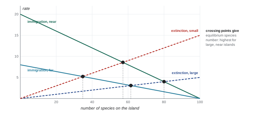
Islands have long fascinated ecologists because they are natural experiments in colonization and extinction. Two patterns are almost universal: larger islands have more species, and islands farther from the mainland have fewer. The species–area relationship, introduced in BIOL-108, describes the first: \( S = cA^z \), with \( z \) typically between 0.2 and 0.35 for islands. In 1963 and 1967, Robert MacArthur and E. O. Wilson proposed the equilibrium theory of island biogeography to explain both patterns. The number of species on an island reflects a balance between the immigration of new species from the mainland and the extinction of species already present. Immigration rate falls as the island fills, because fewer arriving species are new; extinction rate rises, because more species are present to go extinct and each has a smaller population. The equilibrium number of species is where the curves cross. Near islands have higher immigration than far islands, and large islands have lower extinction than small ones, because their populations are larger.
import numpy as np
from scipy.optimize import brentq

P = 100                                   # species in the mainland pool
def immigration(S, I0): return I0 * (1 - S / P)
def extinction(S, E0): return E0 * S / P

for label, I0, E0 in [("large near", 20, 5), ("large far", 8, 5),
                      ("small near", 20, 15), ("small far", 8, 15)]:
    S_eq = brentq(lambda S: immigration(S, I0) - extinction(S, E0), 0, P)
    turnover = immigration(S_eq, I0)
print(f"{label:10s}: equilibrium S = {S_eq:5.1f} species, turnover {turnover:4.1f} species per unit time")large near: equilibrium S = 80.0 species, turnover 4.0 species per unit time large far : equilibrium S = 61.5 species, turnover 3.1 species per unit time small near: equilibrium S = 57.1 species, turnover 8.6 species per unit time small far : equilibrium S = 34.8 species, turnover 5.2 species per unit time
The theory also predicts ongoing turnover: species keep arriving and disappearing even at equilibrium. In 1969, Daniel Simberloff and Wilson tested it by fumigating six tiny mangrove islands in the Florida Keys to remove all insects and spiders, then watching recolonization. Within about a year, species numbers returned close to their original levels, with the nearest islands gaining the most, though the species composition was different, consistent with an equilibrium of numbers maintained by turnover.
Island biogeography applies to any isolated habitat: lakes in a forest, mountaintops above treeline (sky islands), caves, and fragments of forest in farmland. It influenced the design of nature reserves and the debate over whether a single large reserve or several small ones of the same total area protect more species. Mountaintop mammals in the Great Basin, studied by James Brown, have been losing species since the end of the last glaciation without recolonization, behaving like islands with no immigration. BIOL-367 applies these ideas to reserve design.
Common mistakes
MistakeSuccession always ends in the same climax community for a given climate.
InsteadCommunities are loosely organized; outcomes depend on history, chance arrivals and disturbance, forming shifting mosaics.
MistakeDisturbance is always harmful to ecosystems.
InsteadMany ecosystems, such as boreal forests and prairies, depend on recurring disturbance like fire.
MistakeEarly species always prepare the way for later ones.
InsteadFacilitation is one mechanism; tolerance and inhibition also operate.
MistakeIslands reach equilibrium when no species move.
InsteadEquilibrium is dynamic, maintained by continuing immigration and extinction (turnover).
MistakeThe intermediate disturbance hypothesis is a universal law.
InsteadMany studies do not find the predicted peak in diversity; it applies to some systems only.
Summary and key terms
- Primary succession starts without soil; secondary succession starts where soil and propagules remain.
- Glacier Bay and Mount St. Helens show succession shaped by nitrogen fixers, biological legacies and chance arrival.
- Connell and Slatyer described facilitation, tolerance and inhibition models; pioneer and late-successional species differ in traits.
- Markov models project succession from replacement probabilities; Gleason's individualistic view replaced Clements's superorganism.
- Disturbance regimes, such as boreal crown fires with serotinous cones, shape communities; fire suppression has altered them.
- The intermediate disturbance hypothesis predicts peak diversity at moderate disturbance but is not universal.
- Island biogeography explains species numbers as a balance of immigration and extinction, with turnover at equilibrium.
- succession
- Directional change in community composition after disturbance.
- primary succession
- Succession on surfaces without soil, such as glacial till or lava.
- secondary succession
- Succession where soil and some organisms remain after disturbance.
- pioneer species
- Early colonists with fast growth and good dispersal.
- facilitation model
- Early species make conditions better for later species.
- climax community
- The relatively stable community once thought to end succession.
- disturbance regime
- The pattern of type, frequency, intensity, size and season of disturbances.
- serotiny
- Retaining seeds in sealed cones or fruits that open after a trigger such as fire.
- fire cycle
- The time needed to burn an area equal to a whole landscape.
- equilibrium theory of island biogeography
- Species number on an island reflects a balance between immigration and extinction.
Practice problems
Work each problem on paper first, then reveal the answer to check.
Is succession after a forest fire primary or secondary? Why?
Show answer
Secondary, because soil, seeds and roots remain.
What role does Sitka alder play at Glacier Bay?
Show answer
It fixes nitrogen and builds soil organic matter, facilitating later species.
Describe the inhibition model of succession.
Show answer
Early species hold the site and resist invasion; later species replace them only when they die.
Give two traits of late-successional plants.
Show answer
Large seeds and high shade tolerance (also slow growth and long life).
Contrast the views of Clements and Gleason.
Show answer
Clements saw communities as integrated superorganisms; Gleason saw them as individual species with overlapping tolerances.
Why do jack pine forests depend on fire?
Show answer
Serotinous cones open in fire, releasing seed onto burned ground where seedlings establish.
With a fire cycle of 100 years, what fraction of forest is older than 100 years?
Show answer
e^(−1) ≈ 0.37.
Why might diversity be low with very rare disturbance?
Show answer
Dominant competitors exclude other species.
In island biogeography, why do larger islands have more species?
Show answer
Larger populations lower extinction rates, raising the equilibrium.
What did the Simberloff and Wilson mangrove experiment show?
Show answer
Species numbers returned to near pre-fumigation levels with different composition, supporting an equilibrium with turnover.
Lesson quiz · 5 questions
Score 60% or more to complete this lesson.
Create a free account to save your progress, take quizzes and earn a certificate.