
BIOL-208 · Lesson 6 of 12 · 25 min
Metapopulations and spatial ecology
So far we have treated a population as if all its members lived in one well-mixed place. Real populations are spread unevenly across landscapes. Individuals cluster where food is rich, avoid one another where they compete, and move between patches of habitat separated by roads, farmland or water. Space changes population dynamics in important ways. A species can persist across a region even though every local population eventually dies out, as long as empty patches are recolonized. Some patches export individuals while others survive only by importing them. This lesson covers how individuals are distributed in space, how ecologists measure it, how populations linked by dispersal behave, and why the arrangement of habitat matters for conservation.
Patterns of dispersion
Dispersion describes how individuals are spaced within a population. Three idealized patterns are recognized. In a random pattern, the position of each individual is independent of the others, as might happen when seeds are scattered by wind onto uniform ground. In a clumped (aggregated) pattern, individuals occur in groups, because resources are patchy, offspring stay near their parents or animals gather for protection; clumping is by far the most common pattern in nature. In a uniform (regular or even) pattern, individuals are more evenly spaced than chance would produce, usually because they compete or defend territories, as with nesting seabirds keeping just beyond pecking distance of their neighbors or desert shrubs whose roots compete for water.
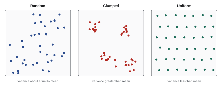
Ecologists test for these patterns by counting individuals in many quadrats of equal size. If individuals are randomly placed, the counts follow a Poisson distribution, for which the variance equals the mean. A variance-to-mean ratio well above 1 indicates clumping, and well below 1 indicates uniformity. A chi-square test checks whether the departure from 1 is larger than chance would produce.
import numpy as np
from scipy import stats

rng = np.random.default_rng(208)
n = 50
samples = {
    "random (Poisson)": rng.poisson(4.0, n),
    "clumped (negative binomial)": rng.negative_binomial(2, 2 / (2 + 4.0), n),
    "uniform (nearly constant)": rng.choice([3, 4, 4, 4, 5], n),
}
for name, counts in samples.items():
    mean, var = counts.mean(), counts.var(ddof=1)
    I = var / mean
    chi2 = I * (n - 1)
    p_hi = stats.chi2.sf(chi2, n - 1); p_lo = stats.chi2.cdf(chi2, n - 1)
    verdict = "clumped" if p_hi < 0.025 else "uniform" if p_lo < 0.025 else "consistent with random"
print(f"{name:28s} mean {mean:4.2f} var {var:5.2f} I = {I:4.2f} -> {verdict}")random (Poisson) mean 4.24 var 4.51 I = 1.06 -> consistent with random clumped (negative binomial) mean 3.16 var 8.79 I = 2.78 -> clumped uniform (nearly constant) mean 4.06 var 0.42 I = 0.10 -> uniform
The pattern detected depends on the scale of sampling. Trees may be uniformly spaced within a small clump but clumped across a hillside. This is another example of the general rule from lesson 1 that ecological patterns change with scale. Field methods for sampling, including quadrats, transects and plotless methods, are covered in BIOL-430.
Home ranges, territories and dispersal
Most animals do not wander at random. A home range is the area an animal uses for its normal activities over a period of time; a territory is the part of it that the animal actively defends against others. Home range size scales with body size and diet: a carnivore must cover more ground than a herbivore of the same mass, because its food is scarcer. A grizzly bear's home range in the Rocky Mountains can exceed 1,000 km² for males, while a deer mouse lives within a few thousand square meters.
Dispersal, the movement of individuals away from where they were born to where they breed, connects populations. Dispersal distances follow a dispersal kernel: most offspring settle close to home, but a few travel much farther. The rare long-distance dispersers matter far more than their numbers suggest, because they colonize new areas and spread genes between populations. Trees migrated northward after the last glaciation faster than average seed dispersal would allow, which ecologists explain by occasional long-distance dispersal by birds and storms, an idea called Reid's paradox.
import numpy as np

rng = np.random.default_rng(208)
# Two kernels with the same mean dispersal distance (100 m)
exp_d = rng.exponential(100, 100_000)
fat_d = rng.lognormal(mean=np.log(100) - 0.5 * 1.3**2, sigma=1.3, size=100_000)
for name, d in [("exponential (thin tail)", exp_d), ("lognormal (fat tail)", fat_d)]:
    print(f"{name:25s} mean {d.mean():6.1f} m  median {np.median(d):6.1f} m  "
f"share beyond 1 km {np.mean(d > 1000) * 100:6.3f}%")exponential (thin tail) mean 99.4 m median 68.4 m share beyond 1 km 0.006% lognormal (fat tail) mean 99.8 m median 42.9 m share beyond 1 km 0.771%
Metapopulations
In 1969, Richard Levins introduced the idea of a metapopulation: a population of populations, each occupying a patch of suitable habitat, connected by dispersal. Local populations go extinct from time to time, through chance or local disasters, and empty patches are recolonized by dispersers from occupied ones. The metapopulation persists if colonization keeps pace with extinction. Levins described this with a remarkably simple model in which \( p \) is the fraction of patches occupied, \( c \) the colonization rate and \( e \) the extinction rate of local populations:
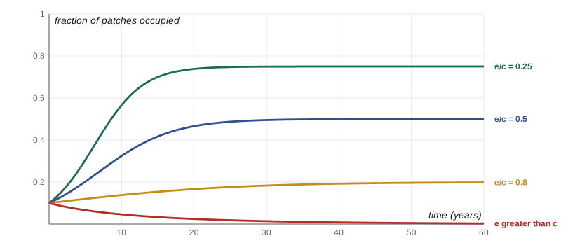
Colonization requires occupied patches to send dispersers (\( p \)) and empty patches to receive them (\( 1 - p \)). At equilibrium, the occupied fraction is \( p^* = 1 - e/c \). The model's key insight is that the metapopulation persists only if \( c > e \), and that a species can disappear from a whole region even while suitable patches remain empty. Destroying some patches lowers the colonization rate, so the occupancy of the remaining patches falls too; if colonization falls below extinction, the metapopulation collapses even though habitat is still present.
import numpy as np

def levins(c, e, p0=0.1, years=60, dt=0.1):
    p = p0
    for _ in range(int(years / dt)):
        p += (c * p * (1 - p) - e * p) * dt
    return p

for c, e in [(0.4, 0.1), (0.4, 0.2), (0.4, 0.32), (0.4, 0.45)]:
    print(f"c = {c}, e = {e}:  p after 60 years = {levins(c, e):.3f}   predicted p* = {max(0, 1 - e / c):.3f}")

# Stochastic version: 40 patches, each occupied or empty
rng = np.random.default_rng(208)
occ = np.zeros(40, bool); occ[:4] = True
history = []
for year in range(50):
    p = occ.mean()
    colonize = (~occ) & (rng.random(40) < 0.4 * p)
    die = occ & (rng.random(40) < 0.15)
    occ = (occ & ~die) | colonize
    history.append(int(occ.sum()))
print("patches occupied, years 1-50:", history[::5])c = 0.4, e = 0.1: p after 60 years = 0.750 predicted p* = 0.750 c = 0.4, e = 0.2: p after 60 years = 0.500 predicted p* = 0.500 c = 0.4, e = 0.32: p after 60 years = 0.198 predicted p* = 0.200 c = 0.4, e = 0.45: p after 60 years = 0.003 predicted p* = 0.000 patches occupied, years 1-50: [4, 4, 3, 1, 1, 4, 3, 4, 20, 20]
The best-studied metapopulation is the Glanville fritillary butterfly on the Åland Islands of Finland, where Ilkka Hanski and colleagues surveyed about 4,000 small meadows every year for decades. Each year roughly a fifth of local populations went extinct and a similar number of empty meadows were colonized. Small, isolated meadows had the highest extinction risk and the lowest chance of colonization, and patch area and isolation predicted occupancy well. These incidence function models, which add patch size and distance to the Levins framework, are now used to plan habitat networks for species such as the Karner blue butterfly in the Great Lakes oak savannas.
Sources and sinks
Patches differ in quality. In a source habitat, births exceed deaths and the local population produces a surplus that emigrates. In a sink habitat, deaths exceed births, and the population persists only because immigrants keep arriving. H. Ronald Pulliam formalized this source–sink idea in 1988. A surprising consequence is that a large fraction of a species' individuals can live in sinks, so counting where animals are found can mislead managers about which habitat matters. Protecting sinks while sources are destroyed leads to collapse. Some habitats are worse than sinks: an ecological trap is a habitat that animals prefer but in which they do poorly, as when mayflies lay eggs on wet-looking asphalt or songbirds nest in hayfields that are mowed before the young fledge.
Worked problem
Source or sink?
In population A, each breeding female produces 1.4 daughters a year; in population B, 0.6. In both, adult survival is 0.5 a year and half of daughters survive their first winter to breed. Ignoring density dependence and migration, which is a source and which a sink?
Show solution
- Each year a female is replaced by herself (if she survives) plus her daughters that survive to breed: λ = adult survival + fecundity × juvenile survival.
- Population A: λ = 0.5 + 1.4 × 0.5 = 1.2.
- Population B: λ = 0.5 + 0.6 × 0.5 = 0.8.
- A grows by 20 percent a year on its own and can export the surplus; B shrinks by 20 percent a year on its own.
Answer: A is a source (λ = 1.2) and B a sink (λ = 0.8). If B has 80 females, it needs about 16 immigrant females a year to hold steady.
Landscapes, fragmentation and corridors
When continuous habitat is broken into smaller, more isolated pieces, a process called fragmentation, metapopulation theory predicts trouble: small patches hold small populations that go extinct more often, and isolation slows recolonization. Fragmentation also increases the amount of edge relative to interior. Edges are often hotter, drier and windier, and they let predators, parasites and invasive species penetrate. Brown-headed cowbirds, which lay their eggs in other birds' nests, thrive along forest edges in eastern North America and reduce the nesting success of forest songbirds in small woodlots.
Connectivity can be restored with habitat corridors or crossing structures. The wildlife overpasses and underpasses on the Trans-Canada Highway in Banff National Park, built since the 1990s, have been used hundreds of thousands of times by animals including grizzly bears, wolves, elk and cougars, and genetic studies show that they help connect bear populations on either side. Similar crossings are now being built across North America. Large-scale conservation initiatives such as the Yellowstone to Yukon Conservation Initiative aim to keep a connected network of habitat along the Rocky Mountains. Lesson 12 returns to fragmentation as one of the main drivers of global change, and BIOL-367 covers reserve design.
| Concept | Key idea | Management implication |
|---|---|---|
| Metapopulation | Local populations blink out and are recolonized | Protect networks of patches, including currently empty ones |
| Source–sink | Some patches export individuals; others depend on immigrants | Identify and protect sources, not just where animals are counted |
| Ecological trap | Animals prefer a habitat where they do poorly | Change the habitat or its attractiveness |
| Edge effects | Conditions and predators differ near edges | Favor large, compact patches |
| Connectivity | Dispersal links patches | Maintain corridors and crossings |
Common mistakes
MistakeRandom dispersion is the most common pattern in nature.
InsteadClumped dispersion is by far the most common, because resources are patchy and offspring stay near parents.
MistakeAn empty habitat patch is useless to a species.
InsteadIn a metapopulation, empty patches are future sites of colonization and are essential for persistence.
MistakeWhere most individuals are found is the most important habitat.
InsteadMany individuals can live in sink habitats that depend on immigrants from sources.
MistakeHabitat loss reduces a metapopulation only by the area lost.
InsteadLosing patches lowers colonization of the remaining ones, so occupancy can collapse while habitat remains.
MistakeAverage dispersal distance determines how fast a species spreads.
InsteadRare long-distance dispersers in the tail of the kernel largely control the rate of spread.
Summary and key terms
- Dispersion can be random, clumped or uniform; clumped is most common. The variance-to-mean ratio of quadrat counts tests the pattern.
- Home ranges and territories reflect body size, diet and competition.
- Dispersal kernels have long tails; rare long-distance dispersers drive colonization and range expansion.
- A metapopulation persists when colonization balances local extinction; in the Levins model p* = 1 − e/c.
- Patch area and isolation predict occupancy, as in the Glanville fritillary.
- Sources produce surplus individuals; sinks depend on immigrants; ecological traps attract animals to poor habitat.
- Fragmentation reduces patch size, increases isolation and edge, and can be offset by corridors and crossings.
- dispersion
- The spatial pattern of individuals within a population.
- variance-to-mean ratio
- An index of dispersion; above 1 suggests clumping and below 1 uniformity.
- home range
- The area an animal uses for its normal activities.
- territory
- An area actively defended against others.
- dispersal kernel
- The probability distribution of distances moved by dispersing individuals.
- metapopulation
- A set of local populations linked by dispersal, with local extinction and recolonization.
- source habitat
- Habitat where births exceed deaths and surplus individuals emigrate.
- sink habitat
- Habitat where deaths exceed births and the population depends on immigration.
- ecological trap
- A habitat that animals prefer but in which they do poorly.
- fragmentation
- The breaking of continuous habitat into smaller, more isolated pieces.
Practice problems
Work each problem on paper first, then reveal the answer to check.
Quadrat counts have mean 5 and variance 12. What pattern is suggested?
Show answer
I = 2.4, well above 1: clumped.
Give two causes of uniform dispersion.
Show answer
Territoriality and competition for water or nutrients.
In the Levins model, c = 0.5 and e = 0.2. What is p*?
Show answer
1 − 0.2/0.5 = 0.6.
What happens to p* if e rises to 0.6 with c = 0.5?
Show answer
p* would be negative, so the metapopulation goes extinct.
Why might protecting only currently occupied patches fail?
Show answer
Empty patches are needed for recolonization; losing them lowers colonization rates.
What two patch properties best predicted Glanville fritillary occupancy?
Show answer
Patch area and isolation.
Define a sink habitat.
Show answer
One where deaths exceed births, so the population persists only with immigration.
Give an example of an ecological trap.
Show answer
Hayfields where grassland birds nest but young are killed by mowing; mayflies laying eggs on asphalt.
How do wildlife crossings in Banff help bear populations?
Show answer
They let bears and other animals cross the highway, connecting populations genetically.
Why do rare long-distance dispersers matter so much?
Show answer
They colonize new areas and connect distant populations, setting the speed of spread.
Lesson quiz · 5 questions
Score 60% or more to complete this lesson.
Create a free account to save your progress, take quizzes and earn a certificate.