
BIOL-201 · Lesson 3 of 12 · 31 min
Probability and statistics in genetics
Genetic predictions are statements of probability. A cross between two heterozygotes does not guarantee that one offspring in four will be recessive; it predicts that, on average, one in four will be. To use genetics in practice, whether in a breeding program, a research laboratory or a genetic counseling session, we need to calculate probabilities for families and samples and to decide whether observed results fit a hypothesis. This lesson develops the product and sum rules, conditional probability, the binomial distribution and the chi-square goodness-of-fit test, the main statistical tools of transmission genetics.
The product and sum rules revisited
Lesson 1 introduced two rules. The product rule gives the probability that independent events all occur: multiply their probabilities. The sum rule gives the probability that any one of several mutually exclusive events occurs: add their probabilities. Most genetics problems combine the two. The trick is to identify which events are independent (different children, different genes that assort independently, egg and sperm) and which outcomes are mutually exclusive (the possible genotypes of a single child).
Worked problem
Combining the rules
Two parents are heterozygous for an autosomal recessive condition (Aa × Aa). What is the probability that their first two children are both unaffected? What is the probability that exactly one of the two is affected?
Show solution
- For each child, P(unaffected) = 3/4 and P(affected) = 1/4, independently of other children.
- Both unaffected: 3/4 × 3/4 = 9/16.
- Exactly one affected can happen two mutually exclusive ways: first affected and second not (1/4 × 3/4), or first not and second affected (3/4 × 1/4).
- Sum rule: 3/16 + 3/16 = 6/16 = 3/8.
Answer: P(both unaffected) = 9/16; P(exactly one affected) = 3/8. The remaining 1/16 is the probability that both are affected, and 9/16 + 6/16 + 1/16 = 1.
A frequent error is to forget that the order of births creates separate outcomes. If a question asks for one affected child among two, the two orders must both be counted. When many children are involved, counting orders by hand becomes tedious, and the binomial distribution does it for us.
The binomial distribution
When each of n independent trials has two outcomes, with probability p for one outcome and q = 1 − p for the other, the probability of exactly k occurrences of the first outcome is given by the binomial formula:
The coefficient \(\binom{n}{k}\), read “n choose k”, counts the number of different orders in which k successes can occur among n trials. In the previous example, n = 2, k = 1, p = 1/4, and \(\binom{2}{1} = 2\), giving \(2 \times \tfrac{1}{4} \times \tfrac{3}{4} = \tfrac{3}{8}\), as before.
Worked problem
A family of five
Two carriers of an autosomal recessive condition plan a family of five children. What is the probability that exactly two are affected? That at least one is affected?
Show solution
- n = 5, p = 1/4 (affected), q = 3/4.
- Number of orders: 5!/(2! 3!) = 10.
- P(exactly 2) = 10 × (1/4)² × (3/4)³ = 10 × 1/16 × 27/64 = 270/1,024 ≈ 0.264.
- P(at least one) = 1 − P(none) = 1 − (3/4)⁵ = 1 − 243/1,024 ≈ 0.763.
Answer: About 26 percent for exactly two affected children, and about 76 percent for at least one.
The “at least one” calculation uses the complement: it is usually easier to calculate the probability that something never happens and subtract from 1 than to add up all the ways it could happen. The code below lists the whole distribution for a family of five.
from math import comb
from fractions import Fraction

p = Fraction(1, 4)          # probability a child is affected (Aa x Aa)
n = 5
print("affected  probability")
for k in range(n + 1):
    pk = comb(n, k) * p**k * (1 - p)**(n - k)
    print(f"{k:5d}     {str(pk):>10s} = {float(pk):.4f}")
print("P(at least one) =", float(1 - (1 - p)**n).__round__(4))affected probability
0 243/1024 = 0.2373
1 405/1024 = 0.3955
2 135/512 = 0.2637
3 45/512 = 0.0879
4 15/1024 = 0.0146
5 1/1024 = 0.0010
P(at least one) = 0.7627Conditional probability
Often we know something that changes the odds. Consider a healthy brother of a child with cystic fibrosis. Both parents must be carriers. Before we know anything about the brother, his chance of being a carrier is 1/2. But we know he is unaffected, which rules out the aa genotype. Among the remaining possibilities, AA (probability 1/4) and Aa (probability 1/2), the carrier genotype is twice as likely. His conditional probability of being a carrier is therefore (1/2) ÷ (3/4) = 2/3, not 1/2.
This 2/3 figure appears constantly in genetic counseling. It is the starting point for calculating risks in later generations, and it illustrates a general principle: probabilities must always be calculated from the information actually available.
Worked problem
Risk to the next generation
The unaffected brother above (carrier probability 2/3) has a child with an unrelated partner from a population in which the carrier frequency is 1/25. What is the probability that the child is affected?
Show solution
- The child is affected only if both parents are carriers and both pass on a.
- P(brother is carrier) = 2/3; P(partner is carrier) = 1/25.
- If both are carriers, P(child aa) = 1/4.
- P = 2/3 × 1/25 × 1/4 = 2/300 = 1/150.
Answer: About 1 in 150, compared with roughly 1 in 2,500 for a random couple in that population (1/25 × 1/25 × 1/4).
Testing hypotheses: observed versus expected
Real data never fit expected ratios exactly. Suppose a cross expected to give a 3 : 1 ratio yields 84 dominant and 36 recessive offspring out of 120. The expected numbers are 90 and 30. Is the difference just chance, or does the hypothesis need revising? Statistics cannot prove a hypothesis true, but it can tell us how often deviations this large would occur by chance if the hypothesis were correct.
The chi-square goodness-of-fit test compares observed (O) and expected (E) counts across all categories:
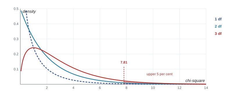
Each term measures how far a category is from expectation, scaled by the expected size so that a difference of 6 matters more in a small class than in a large one. The larger χ², the worse the fit. To interpret χ² we need the degrees of freedom (df), which for a goodness-of-fit test is the number of categories minus one when the expected ratio is specified in advance. We then find the P value: the probability of obtaining a χ² at least this large if the hypothesis is true.
By convention in biology, if P is greater than 0.05 we do not reject the hypothesis: the deviation is consistent with chance. If P is 0.05 or less, the deviation is considered statistically significant and we reject the hypothesis, recognizing that about 1 time in 20 we will reject a correct hypothesis by bad luck. The 0.05 threshold is a convention, not a law of nature, and modern practice favors reporting the P value itself.
| Degrees of freedom | Critical χ² at P = 0.05 | Critical χ² at P = 0.01 |
|---|---|---|
| 1 | 3.84 | 6.63 |
| 2 | 5.99 | 9.21 |
| 3 | 7.81 | 11.34 |
| 4 | 9.49 | 13.28 |
| 5 | 11.07 | 15.09 |
Worked problem
A chi-square test of a 3 : 1 ratio
A cross gives 84 dominant and 36 recessive offspring. Test the fit to 3 : 1.
Show solution
- Expected: 120 × 3/4 = 90 dominant and 120 × 1/4 = 30 recessive.
- χ² = (84 − 90)²/90 + (36 − 30)²/30 = 36/90 + 36/30 = 0.40 + 1.20 = 1.60.
- df = 2 categories − 1 = 1.
- 1.60 is below the critical value 3.84, so P > 0.05 (in fact P ≈ 0.21).
Answer: The data are consistent with a 3 : 1 ratio; a deviation this large would occur by chance about one time in five.
Testing a dihybrid ratio
With four phenotype classes, as in a dihybrid cross, there are 3 degrees of freedom. The code below tests Mendel's own dihybrid data against 9 : 3 : 3 : 1 and then tests an invented data set against the same ratio. In the second case the fit is poor, and the pattern of deviation (too many parental types, too few recombinant types) is a clue that the two genes may be linked, a topic for lesson 8.
from scipy.stats import chisquare

def test(observed, ratio, label):
    n = sum(observed)
    expected = [n * r / sum(ratio) for r in ratio]
    stat, p = chisquare(observed, expected)
    print(label)
    print("  observed:", observed)
    print("  expected:", [round(e, 1) for e in expected])
    print(f"  chi-square = {stat:.2f}, df = {len(observed) - 1}, P = {p:.4f}")

test([315, 108, 101, 32], [9, 3, 3, 1], "Mendel's round/yellow dihybrid F2")
test([620, 112, 105, 163], [9, 3, 3, 1], "Invented F2 for two other genes")Mendel's round/yellow dihybrid F2 observed: [315, 108, 101, 32] expected: [312.8, 104.2, 104.2, 34.8] chi-square = 0.47, df = 3, P = 0.9254 Invented F2 for two other genes observed: [620, 112, 105, 163] expected: [562.5, 187.5, 187.5, 62.5] chi-square = 234.18, df = 3, P = 0.0000
Mendel's data fit extraordinarily well, with a χ² of less than 0.5. In 1936 the statistician Ronald Fisher pointed out that, across all of Mendel's experiments, the fit was better than chance alone would usually produce, and suggested the data might have been adjusted, perhaps unconsciously or by an assistant. Later analyses have argued about this conclusion for decades without settling it. Whatever happened, the ratios Mendel reported have been confirmed many times by others.
Using chi-square correctly
The chi-square test has rules that are easy to forget. It must be applied to counts, never to percentages or proportions, because the size of the sample matters: 30 : 10 and 300 : 100 have the same proportions but very different reliability. Expected counts should generally be at least 5 in every category; with smaller samples, an exact test such as the binomial test is better. And a non-significant result does not prove the hypothesis is right; it means only that the data do not give strong evidence against it. Small samples often fail to reject quite wrong hypotheses.
| Situation | Correct approach |
|---|---|
| Data given as percentages | Convert back to counts before calculating χ² |
| An expected class has fewer than 5 | Combine classes if biologically sensible, or use an exact test |
| Ratio predicted in advance (for example 9 : 3 : 3 : 1) | df = number of classes − 1 |
| Parameter estimated from the same data (for example an allele frequency) | Subtract one more degree of freedom for each estimated parameter |
| P > 0.05 | “Do not reject”; the data are consistent with the hypothesis, not proof of it |
Sample size and power
How many offspring should a breeder count to be confident of distinguishing a 3 : 1 ratio from, say, a 1 : 1 ratio? The ability of a test to detect a real difference is called its power. Power rises with sample size. The simulation below repeatedly samples families from a true 1 : 1 ratio and tests them against 3 : 1, recording how often the false 3 : 1 hypothesis is correctly rejected.
import numpy as np
from scipy.stats import chisquare
rng = np.random.default_rng(201)

def power(n, true_p=0.5, null_p=0.75, reps=2000):
    rejected = 0
    for _ in range(reps):
        dom = rng.binomial(n, true_p)
        stat, p = chisquare([dom, n - dom], [n * null_p, n * (1 - null_p)])
        rejected += p <= 0.05
    return rejected / reps

for n in (8, 16, 32, 64, 128):
print(f"n = {n:3d}: false 3:1 hypothesis rejected in {power(n):.1%} of samples")n = 8: false 3:1 hypothesis rejected in 36.8% of samples n = 16: false 3:1 hypothesis rejected in 59.4% of samples n = 32: false 3:1 hypothesis rejected in 90.0% of samples n = 64: false 3:1 hypothesis rejected in 99.1% of samples n = 128: false 3:1 hypothesis rejected in 100.0% of samples
With 8 offspring the wrong hypothesis is rejected less than half the time; with 64 it is rejected almost always. This is a practical reason why geneticists prefer organisms with large broods, and why conclusions from small human families must be pooled across many families before they are trustworthy.
Common mistakes
MistakeFor two children of carriers, P(exactly one affected) = 1/4 × 3/4 = 3/16.
InsteadThere are two birth orders, so P = 2 × 3/16 = 3/8.
MistakeAn unaffected sibling of a child with a recessive condition has a 1/2 chance of being a carrier.
InsteadKnowing the sibling is unaffected removes the aa class, so the carrier probability is 2/3.
MistakeChi-square can be calculated directly from percentages.
InsteadIt must use actual counts, because sample size affects reliability.
MistakeA P value above 0.05 proves the hypothesis is correct.
InsteadIt means the data are consistent with the hypothesis; they do not prove it, especially with small samples.
MistakeDegrees of freedom equal the number of offspring minus one.
InsteadFor a goodness-of-fit test, df is the number of categories minus one (minus any parameters estimated from the data).
Summary and key terms
- Multiply probabilities of independent events; add probabilities of mutually exclusive outcomes, remembering different birth orders.
- The binomial formula gives the probability of k outcomes of one type in n independent trials.
- Use the complement, 1 − P(none), for “at least one” questions.
- Conditional probability uses known information: an unaffected sibling of an affected child has a 2/3 carrier probability.
- The chi-square goodness-of-fit test compares observed and expected counts; df is the number of classes minus one.
- P ≤ 0.05 conventionally leads to rejecting a hypothesis; P > 0.05 means the data are consistent with it.
- Statistical power increases with sample size, so small samples can fail to detect wrong hypotheses.
- independent events
- Events whose outcomes do not affect each other’s probabilities.
- mutually exclusive
- Outcomes that cannot occur together.
- binomial distribution
- The probability distribution of the number of successes in n independent two-outcome trials.
- complement
- The event that a given event does not occur; P(not A) = 1 − P(A).
- conditional probability
- The probability of an event given that another event is known to have occurred.
- chi-square test
- A statistical test comparing observed and expected counts.
- degrees of freedom
- The number of independent values free to vary; for goodness of fit, the number of classes minus one.
- P value
- The probability of a result at least as extreme as the one observed if the hypothesis were true.
- null hypothesis
- The hypothesis being tested, typically that observed differences are due to chance.
- statistical power
- The probability that a test will detect a real deviation from the hypothesis.
Practice problems
Work each problem on paper first, then reveal the answer to check.
Two carriers of a recessive condition have three children. What is the probability all three are unaffected?
Show answer
(3/4)³ = 27/64 ≈ 0.42.
For the same couple, what is the probability that exactly one of three children is affected?
Show answer
3 × (1/4) × (3/4)² = 27/64 ≈ 0.42.
What is the probability that at least one of four children of two carriers is affected?
Show answer
1 − (3/4)⁴ = 1 − 81/256 ≈ 0.68.
A woman’s brother has a recessive condition; her parents are unaffected. What is her probability of being a carrier?
Show answer
2/3.
Calculate χ² for observed 60 : 40 against an expected 1 : 1 ratio.
Show answer
Expected 50 : 50; χ² = 100/50 + 100/50 = 4.0; df = 1; P < 0.05, so reject 1 : 1.
How many degrees of freedom are there when testing a 1 : 2 : 1 ratio?
Show answer
Two.
Why should χ² not be calculated from percentages?
Show answer
Because it depends on sample size; percentages hide the number of observations.
A test gives χ² = 5.2 with 3 df. Do you reject the hypothesis at P = 0.05?
Show answer
No; 5.2 is below the critical value 7.81.
What does a P value of 0.30 mean?
Show answer
If the hypothesis were true, deviations at least this large would occur about 30 percent of the time; there is no evidence against it.
Why do small samples often fail to reject a wrong hypothesis?
Show answer
Because their power is low; random variation can easily mask the real difference.
Lesson quiz · 5 questions
Score 60% or more to complete this lesson.
Create a free account to save your progress, take quizzes and earn a certificate.