
STAT-252 · Lesson 9 of 12 · 22 min
Hypothesis testing and the Neyman–Pearson lemma
A hypothesis test is a rule for deciding, from data, whether to reject a statement about a parameter. Significance tests in the form of tail probabilities go back to John Arbuthnot's 1710 analysis of christening records and to Karl Pearson's chi-square test of 1900, and Fisher made the p-value central in his 1925 book Statistical Methods for Research Workers. Jerzy Neyman and Egon Pearson gave testing a decision-theoretic footing in their 1933 paper On the problem of the most efficient tests of statistical hypotheses, which introduced the two types of error, the power function and the fundamental lemma that bears their names. This lesson develops that theory, shows how it identifies optimal tests, and explains what p-values do and do not mean.
The framework
A test compares a null hypothesis \(H_0: \theta \in \Theta_0\) with an alternative \(H_1: \theta \in \Theta_1\), where \(\Theta_0\) and \(\Theta_1\) are disjoint subsets of the parameter space. A hypothesis that specifies a single distribution, such as \(\mu = 500\), is simple; one that allows several, such as \(\mu < 500\), is composite. The test is defined by a rejection region \(R\): reject \(H_0\) if the data fall in \(R\), and otherwise do not reject it. Usually \(R\) is described through a test statistic \(T(X)\) and a critical value \(c\), as in reject if \(T > c\).
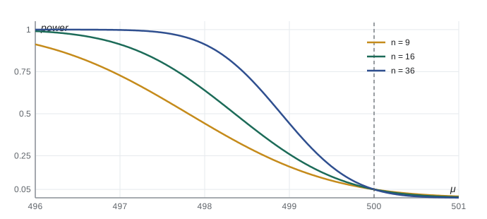
Two kinds of mistake are possible. A type I error rejects a true null; a type II error fails to reject a false one. The power function \(\beta(\theta) = P_\theta(X \in R)\) gives the probability of rejection at each parameter value. For \(\theta \in \Theta_0\) it is the type I error probability, and for \(\theta \in \Theta_1\) it is the power, one minus the type II error probability. The size of the test is \(\sup_{\theta \in \Theta_0}\beta(\theta)\), and a test has level \(\alpha\) if its size is at most \(\alpha\).
The two error probabilities pull against each other: enlarging \(R\) reduces type II errors and increases type I errors. Neyman and Pearson resolved the conflict by treating the hypotheses asymmetrically. Fix the type I error rate at a small level \(\alpha\), conventionally 0.05 or 0.01, and among tests with that level choose the one with the greatest power. The null hypothesis is the claim that should not be rejected without strong evidence: a new drug is no better than the old one, a machine is correctly calibrated, a defendant is innocent.
Worked problem
Is the filling machine underfilling?
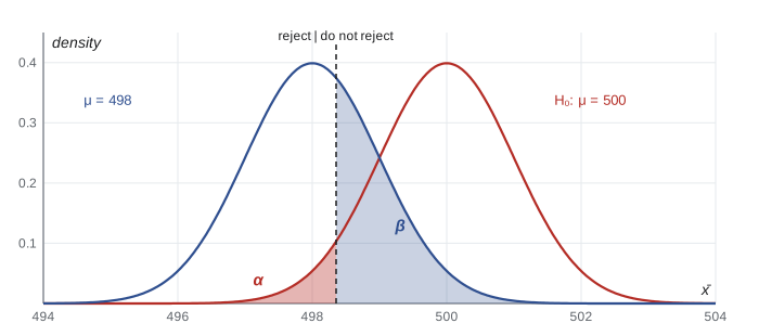
A machine fills bottles with a nominal 500 ml. Fills are normal with \(\sigma = 4\) ml. From 16 bottles, test \(H_0: \mu = 500\) against \(H_1: \mu < 500\) at level 0.05, and find the power when \(\mu = 498\).
Show solution
- Under \(H_0\), \(\bar X \sim N(500, 1)\), since \(\sigma/\sqrt n = 4/4 = 1\).
- Reject when \(\bar X < 500 - 1.645 \times 1 = 498.355\); this has probability 0.05 under \(H_0\).
- If \(\mu = 498\), then \(\bar X \sim N(498, 1)\) and the power is \(P(\bar X < 498.355) = \Phi(0.355) \approx 0.639\).
- To have power 0.9 at \(\mu = 498\), we need \(1.645 + 1.282 \le 2\sqrt n/4\), so \(\sqrt n \ge 5.853\) and \(n \ge 34.3\), that is 35 bottles.
Answer: Reject \(H_0\) if the mean of 16 fills is below 498.36 ml. A real shortfall of 2 ml would be detected only about 64% of the time; 35 bottles would raise this to 90%.
The Neyman–Pearson lemma
For two simple hypotheses, the best test has a remarkably clean form. Suppose \(H_0: \theta = \theta_0\) and \(H_1: \theta = \theta_1\), with likelihoods \(L_0(x)\) and \(L_1(x)\). The Neyman–Pearson lemma says that the test that rejects \(H_0\) when
where \(k\) is chosen so that the size is exactly \(\alpha\), is a most powerful test of level \(\alpha\): no other test with size at most \(\alpha\) has greater power at \(\theta_1\).
The proof is short. Let \(\phi\) be the indicator of the likelihood ratio test's rejection region and \(\psi\) that of any other level-\(\alpha\) test. Wherever \(\phi = 1\), \(L_1 - kL_0 > 0\) and \(\phi - \psi \ge 0\); wherever \(\phi = 0\), \(L_1 - kL_0 \le 0\) and \(\phi - \psi \le 0\). So \((\phi - \psi)(L_1 - kL_0) \ge 0\) everywhere, and integrating gives
Since \(E_0[\phi] = \alpha \ge E_0[\psi]\), the second bracket is non-negative, so \(E_1[\phi] \ge E_1[\psi]\): the likelihood ratio test has at least as much power. The idea is intuitive. Each possible data point costs some type I error probability, \(L_0(x)\), and buys some power, \(L_1(x)\). With a fixed budget \(\alpha\), the best buy is to include the points with the highest ratio of power to cost.
For the normal mean with \(\theta_1 < \theta_0\), the ratio \(L_1/L_0 = \exp\{n(\theta_1 - \theta_0)\bar x/\sigma^2 + \text{const}\}\) is a decreasing function of \(\bar x\), so rejecting for a large ratio is the same as rejecting for small \(\bar x\). The bottling test is therefore most powerful against \(\mu = 498\).
Discrete data and randomization
With discrete data, a size of exactly 0.05 may be impossible. Testing \(H_0: \lambda = 2\) against \(\lambda > 2\) from one Poisson count, the tail probabilities are \(P(X \ge 5) \approx 0.053\) and \(P(X \ge 6) \approx 0.017\). Neyman and Pearson's theory allows a randomized test that rejects when \(X \ge 6\) and, when \(X = 5\), rejects with a probability chosen to make the size exactly 0.05. Randomized tests settle theoretical questions but are almost never used in practice: no scientist would accept a conclusion that depended on a coin toss after the data were in. Practitioners use the conservative test with size 0.017, or report the p-value.
Uniformly most powerful tests
For composite alternatives, a uniformly most powerful (UMP) test is one that is most powerful against every \(\theta \in \Theta_1\) at once. Such tests exist for one-sided hypotheses in families with a monotone likelihood ratio: families in which \(L(\theta_2)/L(\theta_1)\) is an increasing function of a statistic \(T\) whenever \(\theta_2 > \theta_1\). The Karlin–Rubin theorem of 1956 then says that rejecting \(H_0: \theta \le \theta_0\) for large \(T\) is UMP against \(H_1: \theta > \theta_0\). All one-parameter exponential families with an increasing natural parameter have this property, including the binomial, Poisson, exponential and normal with known variance.
For two-sided alternatives, such as \(\mu \ne 500\), no UMP test exists. The most powerful test against \(\mu = 498\) rejects for small \(\bar x\), while the most powerful test against \(\mu = 502\) rejects for large \(\bar x\), and no single test can do both. The usual two-sided test, which rejects when \(|\bar x - 500| > 1.96\sigma/\sqrt n\), is a compromise. It is UMP among unbiased tests, those whose power is never less than \(\alpha\) on the alternative.
p-values
Rather than report only reject or do not reject at a fixed level, it is more informative to report the p-value: the smallest level at which the observed data would lead to rejection. Equivalently, for a test that rejects for large \(T\), the p-value is \(P_{H_0}(T \ge t_{\text{obs}})\), the probability under the null of a result at least as extreme as the one observed. If \(\bar x = 498.1\) for the bottling machine, the p-value is \(\Phi(-1.9) \approx 0.029\). A level-\(\alpha\) test rejects exactly when the p-value is at most \(\alpha\).
When the null is simple and the test statistic is continuous, the p-value is uniformly distributed on \((0, 1)\) under the null, by the probability integral transform. This is what makes it a calibrated measure: under \(H_0\), a p-value below 0.05 occurs 5% of the time. Under an alternative, small p-values become more likely, and the distribution piles up near zero.
p-values are frequently misread. A p-value is not the probability that the null hypothesis is true, nor the probability that the result was due to chance. It says nothing about the size of an effect: with enough data, a trivial difference produces a tiny p-value, and with too little data, an important effect may not reach significance. A p-value above 0.05 is not evidence that the null is true. The American Statistical Association published a statement on these points in 2016, recommending that p-values be reported with effect sizes and confidence intervals and not used as the sole basis for a conclusion.
Two philosophies in one procedure
Modern practice blends two views that their originators regarded as incompatible. For Fisher, a significance test measured the strength of evidence against a single null hypothesis, with no alternative formally specified; the p-value was a graded measure, and a small one meant that either something unusual had happened or the hypothesis was false. For Neyman and Pearson, a test was a rule of behaviour with known long-run error rates, chosen by its power against a specified alternative, and the output was a decision, not a degree of evidence. Fisher objected that scientific inference is not acceptance sampling in a factory, and Neyman replied that Fisher's tests had no principled way to choose a statistic. The usual textbook procedure, in which an alternative and a level are fixed in advance but an exact p-value is also reported, takes something from each. Knowing the two origins helps explain why the p-value cannot be read as an error rate for the particular study at hand.
Many tests at once
If 20 independent true null hypotheses are each tested at level 0.05, the chance of at least one false rejection is \(1 - 0.95^{20} \approx 0.64\). Testing many hypotheses, whether many genes, many subgroups or many outcomes, inflates false discoveries. The Bonferroni correction tests each of \(m\) hypotheses at level \(\alpha/m\), which keeps the probability of any false rejection at most \(\alpha\) by Boole's inequality. Yoav Benjamini and Yosef Hochberg's 1995 procedure controls instead the false discovery rate, the expected proportion of false rejections among all rejections, and is more powerful when many effects are real.
import math, random
from statistics import NormalDist

Z = NormalDist()
# bottling test: critical value, power and sample size
c = 500 - 1.645 * 4 / math.sqrt(16)
print(f"critical value {c:.3f}")
for n in (9, 16, 36):
    se = 4 / math.sqrt(n); cn = 500 - 1.645 * se
    print(f"n = {n:2d}: power at mu = 498 is {Z.cdf((cn - 498) / se):.3f}")
n_needed = math.ceil(((1.645 + Z.inv_cdf(0.9)) * 4 / 2) ** 2)
print(f"sample size for power 0.9 at 498: {n_needed}")

# Poisson tail probabilities for the discrete test
pois = lambda k, lam: math.exp(-lam) * lam ** k / math.factorial(k)
for c0 in (5, 6):
    print(f"P(X >= {c0} | lambda = 2) = {1 - sum(pois(k, 2) for k in range(c0)):.4f}")

# p-values are uniform under the null, and pile up near 0 under an alternative
rng = random.Random(9)
def pval(mu, n=16):
    xbar = sum(rng.gauss(mu, 4) for _ in range(n)) / n
    return Z.cdf((xbar - 500) / 1.0)
for mu in (500, 498):
    ps = [pval(mu) for _ in range(10000)]
    share = [sum(p < t for p in ps) / len(ps) for t in (0.01, 0.05, 0.5)]
    print(f"mu = {mu}: P(p < 0.01) {share[0]:.3f}, P(p < 0.05) {share[1]:.3f}, P(p < 0.5) {share[2]:.3f}")
print(f"chance of a false rejection among 20 true nulls: {1 - 0.95 ** 20:.3f}")critical value 498.355 n = 9: power at mu = 498 is 0.442 n = 16: power at mu = 498 is 0.639 n = 36: power at mu = 498 is 0.912 sample size for power 0.9 at 498: 35 P(X >= 5 | lambda = 2) = 0.0527 P(X >= 6 | lambda = 2) = 0.0166 mu = 500: P(p < 0.01) 0.010, P(p < 0.05) 0.047, P(p < 0.5) 0.496 mu = 498: P(p < 0.01) 0.376, P(p < 0.05) 0.644, P(p < 0.5) 0.977 chance of a false rejection among 20 true nulls: 0.642
Under the null mean of 500, the simulated p-values fall below 0.01, 0.05 and 0.5 in close to 1%, 5% and 50% of samples, as uniformity requires. When the true mean is 498, the share below 0.05 is close to the power of 0.64 computed in the worked example. The power calculation also shows the cost of small samples: with 9 bottles a 2 ml shortfall is caught less than half the time.
Common mistakes
MistakeInterpreting the p-value as the probability that the null hypothesis is true.
InsteadIt is the probability, computed assuming the null, of data at least as extreme as those observed.
MistakeConcluding that the null is true because the test did not reject.
InsteadFailure to reject may reflect low power; report an interval to show which values remain plausible.
MistakeTreating statistical significance as practical importance.
InsteadA tiny effect can be highly significant with a large sample; report the estimated effect and its interval.
MistakeChoosing a one-sided alternative after seeing the data.
InsteadThe direction must be fixed in advance, or the actual type I error rate doubles.
MistakeTesting many hypotheses without adjustment.
InsteadUse Bonferroni or false discovery rate control when many tests are run.
Summary and key terms
- A test specifies a rejection region; type I error rejects a true \(H_0\), type II error fails to reject a false one.
- The power function \(\beta(\theta)\) is the probability of rejection at each \(\theta\); the size is its maximum over \(\Theta_0\).
- Neyman–Pearson lemma: for simple hypotheses, rejecting for a large likelihood ratio is most powerful.
- UMP tests exist for one-sided alternatives in families with monotone likelihood ratio, not for two-sided ones.
- The p-value is the smallest level at which the data would reject; it is uniform under a simple null.
- Multiple testing requires adjustment, such as Bonferroni or false discovery rate control.
- null hypothesis
- The statement tested, rejected only on strong evidence.
- type I error
- Rejecting a true null hypothesis.
- type II error
- Failing to reject a false null hypothesis.
- power
- The probability of rejecting the null when an alternative is true.
- size
- The maximum type I error probability over the null hypothesis.
- most powerful test
- The test with the greatest power at a given alternative among tests of the same level.
- monotone likelihood ratio
- A family in which the likelihood ratio is increasing in a statistic.
- p-value
- The probability under the null of a result at least as extreme as the one observed.
Practice problems
Work each problem on paper first, then reveal the answer to check.
For the bottling test with 16 bottles, find the power when \(\mu = 497\).
Show answer
\(\Phi((498.355 - 497)/1) = \Phi(1.355) \approx 0.912\).
Derive the most powerful test of \(\lambda = 1\) against \(\lambda = 2\) for an exponential sample.
Show answer
\(L_1/L_0 = 2^n e^{-\sum x_i}\), which is decreasing in \(\sum x_i\), so reject when \(\sum X_i\) is small; the critical value comes from \(2\sum X_i \sim \chi^2_{2n}\) under \(H_0\).
A two-sided z test gives \(z = 2.3\). What is the p-value?
Show answer
\(2(1 - \Phi(2.3)) \approx 2 \times 0.0107 = 0.021\).
Why is there no UMP test of \(\mu = 0\) against \(\mu \ne 0\) for a normal mean?
Show answer
The most powerful tests against positive and against negative alternatives reject in opposite tails.
You run 10 tests and want overall type I error at most 0.05. What level does Bonferroni use for each?
Show answer
0.005.
Show that the binomial family has a monotone likelihood ratio in \(X\).
Show answer
For \(p_2 > p_1\), \(L(p_2)/L(p_1) = (p_2/p_1)^x((1 - p_2)/(1 - p_1))^{n - x}\), which is increasing in \(x\).
Lesson quiz · 5 questions
Score 60% or more to complete this lesson.
Create a free account to save your progress, take quizzes and earn a certificate.