Likelihood ratio tests

The Neyman–Pearson lemma gives the best test for two simple hypotheses, and lesson 9 showed that optimal tests exist in a few other cases. Most real questions are more complicated: the null hypothesis is composite, there are nuisance parameters, and the alternative may involve several parameters at once. The generalized likelihood ratio test extends the lemma's idea to all of these settings by comparing the best fit under the null with the best fit overall. Neyman and Pearson proposed it in 1928, and Samuel Wilks proved in 1938 that its statistic has an approximate chi-square distribution in large samples, which made it usable almost everywhere. Together with the closely related score and Wald tests, it is the standard machinery behind the tests reported by regression software, the chi-square tests for tables, and model comparison in general.

The generalized likelihood ratio

To test \(H_0: \theta \in \Theta_0\) against \(H_1: \theta \in \Theta \setminus \Theta_0\), compute

where \(\hat\theta_0\) is the MLE under the null, the restricted MLE, and \(\hat\theta\) is the unrestricted MLE. Because the denominator maximizes over a larger set, \(0 \le \Lambda \le 1\). A value near 1 means the null fits nearly as well as the best model; a small value means the data are much more probable under some alternative. The test rejects \(H_0\) when \(\Lambda\) is small, or equivalently when the deviance-type statistic

is large. When both hypotheses are simple, this is the Neyman–Pearson test. In other cases it is not guaranteed to be optimal, but it usually performs very well and has the great advantage of being defined for any model with a likelihood.

Example: the t test is a likelihood ratio test

Let \(X_1, \ldots, X_n\) be normal with both parameters unknown, and test \(H_0: \mu = \mu_0\). The unrestricted MLEs are \(\bar x\) and \(\hat\sigma^2 = \frac1n\sum(x_i - \bar x)^2\); under the null, \(\hat\sigma_0^2 = \frac1n\sum(x_i - \mu_0)^2\). Substituting into the normal likelihood, the exponential terms both reduce to \(e^{-n/2}\), and

using the identity \(\sum(x_i - \mu_0)^2 = \sum(x_i - \bar x)^2 + n(\bar x - \mu_0)^2\). Since \(\Lambda\) is a decreasing function of \(|T|\), the likelihood ratio test is exactly the two-sided \(t\) test, and the exact \(t_{n-1}\) distribution gives its critical values. Many classical tests, including the \(F\) test of lesson 11, arise in the same way, so the likelihood ratio principle unifies them.

Wilks's theorem

Usually the exact distribution of \(\Lambda\) is not available. Wilks's theorem supplies an approximation: under the regularity conditions of lesson 6, if \(H_0\) is true and fixes \(r\) of the parameters (so the dimension of \(\Theta_0\) is \(r\) less than that of \(\Theta\)), then

The degrees of freedom equal the number of free parameters under the alternative minus the number under the null. For one parameter, the result follows from a second-order expansion: \(\ell(\theta_0) \approx \ell(\hat\theta) - \frac12 J(\hat\theta)(\hat\theta - \theta_0)^2\), so \(-2\log\Lambda \approx J(\hat\theta)(\hat\theta - \theta_0)^2\), the square of an approximately standard normal variable. A test at level 0.05 with one degree of freedom rejects when \(-2\log\Lambda > 3.84\).

Goodness of fit and contingency tables

For multinomial counts \(O_1, \ldots, O_k\) in \(k\) categories, a null hypothesis specifies category probabilities \(p_j(\theta)\), possibly depending on \(q\) estimated parameters. The likelihood ratio statistic is

and it is approximately \(\chi^2_{k-1-q}\). Karl Pearson's 1900 statistic \(X^2 = \sum(O_j - E_j)^2/E_j\) is a quadratic approximation to \(G^2\), obtained by expanding the logarithm, and the two usually agree closely. Fisher corrected Pearson's degrees of freedom in 1922 by showing that one degree is lost for each estimated parameter. A common rule of thumb asks for expected counts of at least 5 in most cells; otherwise exact methods or merged categories are safer.

For example, a plant cross predicted to give tall and short offspring in the ratio 3:1 produces 290 tall and 110 short plants out of 400. The expected counts are 300 and 100. Then \(X^2 = 100/300 + 100/100 = 1.33\) and \(G^2 = 2[290\log(290/300) + 110\log(110/100)] \approx 1.31\), each with 1 degree of freedom and a p-value of about 0.25. The data are consistent with the 3:1 ratio.

For an \(r \times c\) contingency table, independence of rows and columns gives expected counts \(E_{ij} = (\text{row total})(\text{column total})/n\), and \(G^2\) or \(X^2\) has \((r - 1)(c - 1)\) degrees of freedom: \(rc - 1\) free cell probabilities under the alternative minus \((r - 1) + (c - 1)\) under independence.

The score and Wald tests

Two asymptotically equivalent alternatives complete what is often called the trinity of likelihood tests. The Wald test, proposed by Abraham Wald in 1943, uses only the unrestricted MLE: \(W = (\hat\theta - \theta_0)^2/\mathrm{se}(\hat\theta)^2\). The score test, proposed by Rao in 1948 and known in econometrics as the Lagrange multiplier test, uses only the restricted fit: \(S = U(\theta_0)^2/(nI(\theta_0))\), which measures how steeply the log-likelihood is still rising at the null value. All three are approximately \(\chi^2_r\) under the null, and they agree in large samples.

In smaller samples they can differ noticeably. The Wald test is not invariant to reparameterization: testing \(\lambda = 1\) and testing \(\log\lambda = 0\) can give different answers. The score test is convenient when the restricted model is easy to fit and the full one is not, as when testing whether extra terms are needed in a regression. Pearson's \(X^2\) is in fact the score test for a multinomial, and the Wilson interval of lesson 8 inverts the score test for a proportion. The likelihood ratio test is invariant and usually the most reliable of the three, at the cost of fitting both models.

Likelihood ratio intervals

Inverting the likelihood ratio test gives a confidence set: all \(\theta_0\) for which \(2[\ell(\hat\theta) - \ell(\theta_0)] \le \chi^2_{1, \alpha}\). For 95% the cut-off is 3.84, so the interval consists of the parameter values whose log-likelihood is within 1.92 of the maximum. Unlike the Wald interval, this interval need not be symmetric, it respects the boundaries of the parameter space, and it is the same whatever parameterization is used.

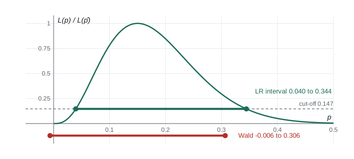
With 3 successes in 20 trials, the likelihood ratio interval runs from about 0.040 to 0.344, skewed to the right as the asymmetric log-likelihood suggests. The Wald interval, \(0.15 \pm 0.156\), runs from below zero to 0.306, an impossible lower end and an upper end that is too low.

Nuisance parameters and the profile likelihood

Most hypotheses concern one parameter while others, called nuisance parameters, must be estimated along the way. In the \(t\) test, \(\sigma\) is a nuisance parameter; in the accident comparison, the common rate is. The likelihood ratio handles them automatically, because both numerator and denominator maximize over every parameter not fixed by the hypothesis. Writing \(\theta = (\psi, \lambda)\) with \(\psi\) of interest, the profile log-likelihood \(\ell_p(\psi) = \max_\lambda \ell(\psi, \lambda)\) replaces each nuisance parameter by its best value for the given \(\psi\). Then \(-2\log\Lambda\) for \(H_0: \psi = \psi_0\) is just \(2[\ell_p(\hat\psi) - \ell_p(\psi_0)]\), and Wilks's theorem applies with as many degrees of freedom as \(\psi\) has components. A profile likelihood interval for \(\psi\) is found exactly as in the one-parameter case, by cutting the profile 1.92 units below its peak. This is how software computes intervals for a single regression coefficient or a gamma shape while accounting for the uncertainty in all the other parameters. When there are many nuisance parameters relative to the sample size, as in the Neyman–Scott problem of lesson 5, the profile likelihood can mislead, and adjusted or conditional likelihoods are needed.

When Wilks's theorem fails

The chi-square approximation needs the null value to lie in the interior of the parameter space. When it lies on the boundary, as in testing whether a variance component is zero or whether a mixture has a second component, the limit changes. For one parameter on the boundary, Steven Self and Kung-Yee Liang showed in 1987 that the limit is an equal mixture of a point mass at 0 and \(\chi^2_1\), so the correct p-value is half the naive one. Wilks's theorem also needs the null model to be nested within the alternative; comparing non-nested models, such as a gamma against a lognormal fit, calls for other tools such as Akaike's information criterion of 1973, \(\mathrm{AIC} = -2\ell(\hat\theta) + 2k\), which penalizes the number of parameters \(k\).

import math
from statistics import NormalDist

Z = NormalDist()
chi2_1_p = lambda g: 2 * (1 - Z.cdf(math.sqrt(g)))     # upper tail of chi-square(1)

# two Poisson rates
x, t = (30, 48), (10, 12)
l0 = sum(x) / sum(t)
G = 2 * sum(xi * math.log(xi / (l0 * ti)) for xi, ti in zip(x, t))
print(f"Poisson rates: pooled {l0:.3f}, G = {G:.3f}, p = {chi2_1_p(G):.3f}")

# goodness of fit to a 3:1 ratio
obs, exp = (290, 110), (300, 100)
X2 = sum((o - e) ** 2 / e for o, e in zip(obs, exp))
G2 = 2 * sum(o * math.log(o / e) for o, e in zip(obs, exp))
print(f"3:1 ratio: X^2 = {X2:.3f} (p {chi2_1_p(X2):.3f}), G^2 = {G2:.3f} (p {chi2_1_p(G2):.3f})")

# the trinity for a proportion: 3 successes in 20, test p = 0.4
k, n, p0 = 3, 20, 0.4
ph = k / n
ll = lambda p: k * math.log(p) + (n - k) * math.log(1 - p)
lrt = 2 * (ll(ph) - ll(p0))
wald = (ph - p0) ** 2 / (ph * (1 - ph) / n)
score = (ph - p0) ** 2 / (p0 * (1 - p0) / n)
print(f"test p = 0.4: LR {lrt:.2f}, Wald {wald:.2f}, score {score:.2f}")

# likelihood ratio interval versus Wald interval
grid = [i / 100000 for i in range(1, 100000)]
inside = [p for p in grid if 2 * (ll(ph) - ll(p)) <= 3.8415]
se = math.sqrt(ph * (1 - ph) / n)
print(f"LR interval {min(inside):.3f} to {max(inside):.3f}; "
      f"Wald interval {ph - 1.96 * se:.3f} to {ph + 1.96 * se:.3f}")

Poisson rates: pooled 3.545, G = 1.557, p = 0.212
3:1 ratio: X^2 = 1.333 (p 0.248), G^2 = 1.305 (p 0.253)
test p = 0.4: LR 5.96, Wald 9.80, score 5.21
LR interval 0.040 to 0.344; Wald interval -0.006 to 0.306

For the test of \(p = 0.4\) with 3 successes in 20, the three statistics differ markedly even though they are asymptotically equivalent. The Wald statistic uses the small estimated variance at \(\hat p = 0.15\) and is the largest; the score statistic uses the variance at \(p = 0.4\) and is the smallest; the likelihood ratio lies between them. All three reject at the 5% level here, but with smaller effects they can disagree, and the likelihood ratio is usually the safest choice.