Point estimators: bias, variance and mean squared error

An estimator is a rule for turning data into a guess at a parameter. There are always many rules to choose from. To estimate the centre of a symmetric distribution we could use the sample mean, the median, the midrange or a trimmed mean; to estimate a variance we could divide the sum of squared deviations by \(n\), by \(n - 1\) or by \(n + 1\). This lesson sets out the criteria for comparing estimators: bias, variance, mean squared error, consistency and efficiency. The criteria are properties of sampling distributions, so they describe how a rule performs on average over many samples, not how close a particular estimate happens to be to the truth.

Bias

Let \(T = T(X_1, \ldots, X_n)\) be an estimator of \(\theta\). Its bias is

and \(T\) is unbiased if the bias is zero for every \(\theta \in \Theta\). The phrase 'for every \(\theta\)' matters: the estimator \(T = 5\) is unbiased when \(\theta = 5\) and badly biased otherwise, and nobody would call it a good estimator. Unbiasedness says that the sampling distribution is centred at the truth, so that over many samples the errors average out. The sample mean is unbiased for the population mean, the sample proportion for a population proportion, and \(\hat F_n(x)\) for \(F(x)\), all by linearity of expectation.

The sample variance \(S^2 = \frac{1}{n-1}\sum (X_i - \bar X)^2\) is unbiased for \(\sigma^2\) for any distribution with a finite variance, not only the normal. The proof uses the decomposition \(\sum (X_i - \mu)^2 = \sum (X_i - \bar X)^2 + n(\bar X - \mu)^2\). Taking expectations, the left side has expectation \(n\sigma^2\) and \(n(\bar X - \mu)^2\) has expectation \(n\operatorname{Var}(\bar X) = \sigma^2\). So \(E[\sum (X_i - \bar X)^2] = (n - 1)\sigma^2\), and dividing by \(n - 1\) gives an unbiased estimator. Dividing by \(n\) gives \(\hat\sigma^2 = \frac{n-1}{n}S^2\), whose bias is \(-\sigma^2/n\): it underestimates on average because the deviations are measured from \(\bar X\), which is closer to the data than \(\mu\) is.

Unbiasedness does not survive nonlinear transformation. Since \(S^2\) is unbiased for \(\sigma^2\) and \(\sqrt{\cdot}\) is concave, Jensen's inequality gives \(E[S] \le \sqrt{E[S^2]} = \sigma\), with strict inequality unless \(S\) is constant. So the sample standard deviation is biased downward. For normal samples the bias factor \(E[S]/\sigma\), called \(c_4\) in quality control, is about 0.94 for \(n = 5\) and 0.99 for \(n = 25\). An unbiased estimator of \(\theta\) gives an unbiased estimator of \(g(\theta)\) only when \(g\) is linear.

Variance and mean squared error

An unbiased estimator can still be useless if it is very variable. The single observation \(X_1\) is unbiased for \(\mu\), but it ignores \(n - 1\) of the observations. The natural measure that combines both kinds of error is the mean squared error

The decomposition follows by adding and subtracting \(E[T]\) inside the square: \((T - \theta)^2 = (T - E[T])^2 + 2(T - E[T])(E[T] - \theta) + (E[T] - \theta)^2\), and the middle term has expectation zero. MSE is the expected squared distance of the estimator from the truth. Its square root, the root mean squared error, is on the scale of the data and is often reported in simulation studies.

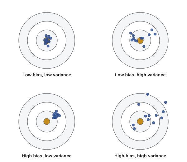
The decomposition explains why a biased estimator can beat an unbiased one: accepting a little bias can buy a large reduction in variance. For a normal sample, consider estimators of \(\sigma^2\) of the form \(c\sum (X_i - \bar X)^2\). Let \(W = \sum(X_i - \bar X)^2\), so \(W/\sigma^2 \sim \chi^2_{n-1}\) with mean \(n - 1\) and variance \(2(n - 1)\). Then \(E[cW] = c(n - 1)\sigma^2\) and \(\operatorname{Var}(cW) = 2c^2(n - 1)\sigma^4\), so

Differentiating in \(c\) and setting the derivative to zero gives \(4c(n - 1) + 2(n - 1)(c(n - 1) - 1) = 0\), so \(c = 1/(n + 1)\). Among estimators of this form, dividing by \(n + 1\) minimizes mean squared error; dividing by \(n\) comes second; the unbiased divisor \(n - 1\) comes last. The differences are small for large \(n\), but the example makes a general point: unbiasedness is one desirable property, not the definition of a good estimator. Ridge regression, shrinkage estimators and much of modern machine learning deliberately trade bias for variance.

Comparing estimators: efficiency

For two unbiased estimators \(T_1\) and \(T_2\), the relative efficiency of \(T_2\) with respect to \(T_1\) is \(\operatorname{Var}(T_1)/\operatorname{Var}(T_2)\). If it is 0.64, then \(T_2\) needs about \(1/0.64 \approx 1.56\) times as many observations to match the precision of \(T_1\). For a normal sample, the sample median has variance approximately \(\pi\sigma^2/(2n)\) for large \(n\), against \(\sigma^2/n\) for the mean, so its efficiency relative to the mean is \(2/\pi \approx 0.64\). That is the price of robustness: the median ignores how far the extreme observations are from the centre, which wastes information when the data really are normal and protects against outliers when they are not. For the double-exponential (Laplace) distribution, whose tails are heavier, the order reverses and the median has efficiency 2 relative to the mean.

The uniform example also shows that the usual \(1/n\) rate is not a law of nature. When the support of the distribution depends on the parameter, estimators can converge faster, and lesson 7 explains why the Cramér–Rao bound does not apply there.

Consistency

A sequence of estimators \(T_n\) is consistent for \(\theta\) if \(T_n \to \theta\) in probability for every \(\theta\): for each \(\varepsilon > 0\), \(P_\theta(|T_n - \theta| > \varepsilon) \to 0\) as \(n \to \infty\). Consistency is the minimal requirement of a sensible estimator: with enough data it should get the answer right. A convenient sufficient condition comes from Chebyshev's inequality applied to \((T_n - \theta)^2\): by Markov's inequality, \(P(|T_n - \theta| > \varepsilon) \le \operatorname{MSE}(T_n)/\varepsilon^2\), so if the MSE tends to zero, the estimator is consistent. In particular, an estimator whose bias and variance both tend to zero is consistent. Thus \(\bar X\), \(S^2\), \(\hat\sigma^2\) and both uniform estimators above are consistent.

The law of large numbers gives consistency of sample moments directly, and the continuous mapping theorem extends it: if \(T_n \to \theta\) in probability and \(g\) is continuous at \(\theta\), then \(g(T_n) \to g(\theta)\) in probability. So \(S = \sqrt{S^2}\) is consistent for \(\sigma\), although it is biased for every \(n\). Consistency and unbiasedness are logically independent. \(X_1\) is unbiased but not consistent; \(\hat\sigma^2\) is biased but consistent.

import random, math
from statistics import mean, median, variance, pvariance

rng = random.Random(252)
n, reps, sigma2 = 10, 40000, 4.0

# three divisors for the variance of a normal sample
res = {"n-1": [], "n": [], "n+1": []}
for _ in range(reps):
    x = [rng.gauss(0, 2) for _ in range(n)]
    w = sum((v - mean(x)) ** 2 for v in x)
    res["n-1"].append(w / (n - 1)); res["n"].append(w / n); res["n+1"].append(w / (n + 1))
print("divisor   bias     variance   MSE")
for k, est in res.items():
    b = mean(est) - sigma2; v = pvariance(est)
    print(f"{k:>5}  {b:+.4f}   {v:.4f}   {v + b * b:.4f}")
print(f"theory MSE: n-1 {2*sigma2**2/(n-1):.4f}, n {(2*(n-1)+1)*sigma2**2/n**2:.4f}, n+1 {2*sigma2**2/(n+1):.4f}")

# mean versus median: normal and Laplace data
def laplace():
    return rng.expovariate(1) * (1 if rng.random() < 0.5 else -1)
for name, gen in (("normal", lambda: rng.gauss(0, 1)), ("Laplace", laplace)):
    ms, md = [], []
    for _ in range(10000):
        x = [gen() for _ in range(51)]
        ms.append(mean(x)); md.append(median(x))
    print(f"{name:>7}: var(mean) {pvariance(ms):.5f}, var(median) {pvariance(md):.5f}, "
          f"efficiency of median {pvariance(ms) / pvariance(md):.2f}")

# uniform endpoint: 2*mean versus (n+1)/n * max
theta, m = 90.0, 28
t1, t2 = [], []
for _ in range(20000):
    x = [rng.uniform(0, theta) for _ in range(m)]
    t1.append(2 * mean(x)); t2.append((m + 1) / m * max(x))
print(f"uniform n={m}: mean T1 {mean(t1):.2f}, T2 {mean(t2):.2f};"
      f" var T1 {pvariance(t1):.2f} (theory {theta**2/(3*m):.2f}), var T2 {pvariance(t2):.2f} (theory {theta**2/(m*(m+2)):.2f})")

divisor   bias     variance   MSE
  n-1  +0.0018   3.5792   3.5792
    n  -0.3984   2.8992   3.0579
  n+1  -0.7258   2.3960   2.9228
theory MSE: n-1 3.5556, n 3.0400, n+1 2.9091
 normal: var(mean) 0.01986, var(median) 0.03076, efficiency of median 0.65
Laplace: var(mean) 0.03830, var(median) 0.02415, efficiency of median 1.59
uniform n=28: mean T1 90.00, T2 90.02; var T1 97.14 (theory 96.43), var T2 9.60 (theory 9.64)

The simulation confirms the algebra: the unbiased divisor has the largest MSE of the three, and dividing by \(n + 1\) has the smallest. The median's efficiency is near 0.64 for normal data and above 1 for the heavier-tailed Laplace data, so which estimator is better depends on the distribution, which is the starting point of robust statistics. For the uniform endpoint the maximum-based estimator's variance is about a tenth of the other's, matching the theory.

No estimator is best everywhere

Why not simply look for the estimator with the smallest MSE? Because MSE is a function of \(\theta\), and two estimators' MSE curves usually cross. The constant estimator \(T = 5\) has MSE \((5 - \theta)^2\), which is zero at \(\theta = 5\), so no estimator can have uniformly smallest MSE unless it is perfect at every parameter value, which is impossible. Statistical theory responds in three ways. The first restricts the class of estimators, for instance to unbiased ones, and then looks for the best within it: lesson 7 shows that among unbiased estimators there is often one with uniformly smallest variance, and gives a lower bound that no unbiased estimator can beat. The second summarizes the MSE curve by a single number, either its maximum over \(\Theta\), which leads to minimax estimators, or its average with respect to a weighting of the parameter values, which leads to Bayes estimators (lesson 12). The third studies large samples, where the comparison simplifies: lesson 6 shows that maximum likelihood estimators are asymptotically unbiased with the smallest possible asymptotic variance under regularity conditions. Squared error is itself a choice. Absolute error \(|T - \theta|\) penalizes large mistakes less severely and leads to medians rather than means; asymmetric losses are natural when overestimating a reserve is cheaper than underestimating it. The choice of loss should come from the problem, but squared error is the default because it is mathematically convenient and leads to the clean variance-plus-bias decomposition.

Standard errors

Reporting an estimate without a measure of its precision is half an answer. The standard error of an estimator is its standard deviation, and in practice we report an estimate of it: \(S/\sqrt n\) for the mean, \(\sqrt{\hat p(1 - \hat p)/n}\) for a proportion. When no formula is available, lesson 8 shows how the bootstrap estimates a standard error by resampling. A standard error answers the question of how much an estimate would vary from sample to sample. It does not include bias, and it does not account for errors that the model leaves out, such as a sample that is not random.