Sampling distributions: chi-square, t and F

When the data are normal, the sample mean and sample variance have exact sampling distributions that underlie the \(t\) test, the chi-square interval for a variance, the \(F\) test and the analysis of variance. This lesson derives them. The route runs through three families built from standard normal variables, the chi-square, \(t\) and \(F\) distributions, and through one remarkable theorem: for a normal sample, \(\bar X\) and \(S^2\) are independent. Independence is what makes the \(t\) statistic work, and it is a property special to the normal distribution.

The chi-square distribution

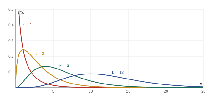
If \(Z_1, \ldots, Z_k\) are independent standard normal variables, the distribution of \(Q = Z_1^2 + \cdots + Z_k^2\) is called chi-square with \(k\) degrees of freedom, written \(\chi^2_k\). For \(k = 1\), STAT-251's transformation methods give the density of \(Z^2\): for \(q > 0\), \(P(Z^2 \le q) = P(-\sqrt q \le Z \le \sqrt q) = 2\Phi(\sqrt q) - 1\), and differentiating gives \(f(q) = q^{-1/2}e^{-q/2}/\sqrt{2\pi}\). This is the gamma density with shape \(1/2\) and rate \(1/2\). Since sums of independent gamma variables with a common rate are gamma with the shapes added (moment generating functions multiply), \(\chi^2_k\) is gamma with shape \(k/2\) and rate \(1/2\):

Its moment generating function is \((1 - 2t)^{-k/2}\) for \(t < 1/2\), its mean is \(k\) and its variance is \(2k\). Each \(Z_i^2\) has mean \(E[Z_i^2] = 1\) and variance \(E[Z_i^4] - 1 = 3 - 1 = 2\), so these also follow directly from linearity and independence. By the central limit theorem, \(\chi^2_k\) is approximately \(N(k, 2k)\) for large \(k\), though the right skew persists for longer than one might expect. Two closure properties follow from the gamma representation: sums of independent chi-square variables are chi-square with the degrees of freedom added, and if \(Q = Q_1 + Q_2\) with \(Q \sim \chi^2_k\), \(Q_1 \sim \chi^2_{k_1}\) and \(Q_1\), \(Q_2\) independent, then \(Q_2 \sim \chi^2_{k - k_1}\), because its mgf must be the ratio of the other two.

The sample variance of a normal sample

Let \(X_1, \ldots, X_n\) be iid \(N(\mu, \sigma^2)\). The central result is the following theorem, sometimes attributed to Cochran in its general form:

The first claim is the closure of the normal family under averaging. For the other two, here is a proof using moment generating functions. Write \(Z_i = (X_i - \mu)/\sigma\), which are iid standard normal. Independence of \(\bar X\) and the vector of deviations \((X_1 - \bar X, \ldots, X_n - \bar X)\) can be shown by computing their joint mgf: for constants \(s\) and \(t_1, \ldots, t_n\), the exponent \(s\bar Z + \sum t_i(Z_i - \bar Z)\) is a linear combination \(\sum a_i Z_i\) with \(a_i = s/n + t_i - \bar t\), where \(\bar t\) is the mean of the \(t_i\). Its mgf is \(\exp(\frac12\sum a_i^2)\). Expanding, \(\sum a_i^2 = s^2/n + \sum (t_i - \bar t)^2\), because the cross term \(\frac{2s}{n}\sum(t_i - \bar t)\) is zero. So the joint mgf factors into a function of \(s\) times a function of the \(t_i\), which proves independence. Since \(S^2\) is a function of the deviations, \(\bar X\) and \(S^2\) are independent.

For the distribution of \(S^2\), start from the identity \(\sum (Z_i - 0)^2 = \sum (Z_i - \bar Z)^2 + n\bar Z^2\), which is the familiar decomposition of a sum of squares about a point into the sum about the mean plus a correction. The left side is \(\chi^2_n\). On the right, \(n\bar Z^2 = (\sqrt n\bar Z)^2\) is \(\chi^2_1\) because \(\sqrt n\bar Z\) is standard normal, and it is independent of the first term by the result just proved. By the closure property, \(\sum (Z_i - \bar Z)^2 = (n-1)S^2/\sigma^2\) is \(\chi^2_{n-1}\). One degree of freedom has been used up in estimating the mean: the \(n\) deviations \(X_i - \bar X\) sum to zero, so only \(n - 1\) of them are free to vary.

Consequences follow at once. Since the mean of \(\chi^2_{n-1}\) is \(n - 1\), \(E[S^2] = \sigma^2\), so dividing by \(n - 1\) rather than \(n\) makes \(S^2\) unbiased, a fact lesson 3 proves without assuming normality. Since the variance of \(\chi^2_{n-1}\) is \(2(n-1)\), \(\operatorname{Var}(S^2) = 2\sigma^4/(n - 1)\). That variance depends heavily on normality. For heavy-tailed data the sample variance is far more variable than this formula suggests, which is why chi-square intervals for a variance are much less robust than \(t\) intervals for a mean.

The independence of \(\bar X\) and \(S^2\) characterizes the normal distribution: for no other distribution are they independent. For an exponential sample, a sample with a large mean tends to have a large variance too, because both are driven by the long right tail. The code below checks this by simulation.

Student's t distribution

If \(Z \sim N(0, 1)\) and \(Q \sim \chi^2_k\) are independent, the distribution of \(T = Z/\sqrt{Q/k}\) is called Student's \(t\) with \(k\) degrees of freedom. Its density, obtained by the transformation method for two variables followed by integrating out \(Q\), is

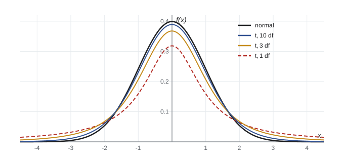
The \(t\) density is symmetric and bell-shaped like the normal but with heavier tails: it decays like \(|t|^{-(k+1)}\) rather than exponentially. Only moments of order less than \(k\) exist. With \(k = 1\) it is the Cauchy distribution, which has no mean at all. As \(k \to \infty\), \(Q/k \to 1\) by the law of large numbers, and \(T\) converges in distribution to \(N(0, 1)\). By \(k = 30\) the two are close in the centre, but tail quantiles still differ: the 0.975 quantile is 2.045 for \(t_{29}\) against 1.960 for the normal.

The application is immediate. For a normal sample, \(Z = \sqrt n(\bar X - \mu)/\sigma\) is standard normal, \(Q = (n-1)S^2/\sigma^2\) is \(\chi^2_{n-1}\), and they are independent. So

The unknown \(\sigma\) has cancelled. This is Gosset's discovery of 1908. Working on small samples of barley and stout at the Guinness brewery in Dublin, he found that replacing \(\sigma\) by \(S\) in the standardized mean produced a distribution with fatter tails than the normal, and that intervals and tests built on the normal were too optimistic for samples of a handful of observations. Fisher later gave the rigorous proof and introduced the degrees-of-freedom parameterization used today.

The F distribution

If \(Q_1 \sim \chi^2_{k_1}\) and \(Q_2 \sim \chi^2_{k_2}\) are independent, the distribution of \(F = (Q_1/k_1)/(Q_2/k_2)\) is called \(F\) with \(k_1\) and \(k_2\) degrees of freedom, named by Snedecor in honour of Fisher. It arises whenever two independent variance estimates are compared. For two independent normal samples of sizes \(m\) and \(n\) with variances \(\sigma_1^2\) and \(\sigma_2^2\), \((S_1^2/\sigma_1^2)/(S_2^2/\sigma_2^2) \sim F_{m-1, n-1}\), which gives a test and an interval for the variance ratio. In the analysis of variance and in regression (lesson 11), the \(F\) statistic compares the variability explained by a model with the variability left over. Three relations are useful: \(1/F \sim F_{k_2, k_1}\), so lower quantiles come from upper ones; the square of a \(t_k\) variable is \(F_{1,k}\); and \(k_1F_{k_1,k_2} \to \chi^2_{k_1}\) as \(k_2 \to \infty\).

import random, math
from statistics import mean, variance

rng = random.Random(252)
def chi2_pdf(q, k):
    return q ** (k / 2 - 1) * math.exp(-q / 2) / (2 ** (k / 2) * math.gamma(k / 2))
def t_pdf(t, k):
    c = math.gamma((k + 1) / 2) / (math.sqrt(k * math.pi) * math.gamma(k / 2))
    return c * (1 + t * t / k) ** (-(k + 1) / 2)

n, reps = 6, 40000
qs, ts, pairs = [], [], []
for _ in range(reps):
    x = [rng.gauss(10, 2) for _ in range(n)]
    m, s2 = mean(x), variance(x)
    qs.append((n - 1) * s2 / 4)
    ts.append((m - 10) / math.sqrt(s2 / n))
    pairs.append((m, s2))
print(f"(n-1)S^2/sigma^2: mean {mean(qs):.3f} (k = {n-1}), var {variance(qs):.3f} (2k = {2*(n-1)})")

# compare a histogram bin with the chi-square density
lo, hi = 3, 4
frac = sum(lo <= q < hi for q in qs) / reps
area = sum(chi2_pdf(lo + (hi - lo) * (i + 0.5) / 200, n - 1) for i in range(200)) * (hi - lo) / 200
print(f"P({lo} <= Q < {hi}): simulated {frac:.4f}, chi-square(5) {area:.4f}")

# t statistic: tail beyond 2.571 (the 0.975 quantile of t_5) versus normal tail
tail = sum(abs(t) > 2.571 for t in ts) / reps
print(f"P(|T| > 2.571): simulated {tail:.4f}, t_5 theory 0.0500, normal would give {2 * (1 - 0.99493):.4f}")
print(f"t_5 density at 0: {t_pdf(0, 5):.4f}   normal density at 0: {1 / math.sqrt(2 * math.pi):.4f}")

# independence of mean and variance: correlation, normal versus exponential
def corr(pr):
    a = [p[0] for p in pr]; b = [p[1] for p in pr]
    ma, mb = mean(a), mean(b)
    num = sum((u - ma) * (v - mb) for u, v in pr)
    return num / math.sqrt(sum((u - ma) ** 2 for u in a) * sum((v - mb) ** 2 for v in b))
expo = []
for _ in range(reps):
    x = [rng.expovariate(1) for _ in range(n)]
    expo.append((mean(x), variance(x)))
print(f"corr(mean, S^2): normal {corr(pairs):+.3f}, exponential {corr(expo):+.3f}")

(n-1)S^2/sigma^2: mean 4.970 (k = 5), var 9.990 (2k = 10)
P(3 <= Q < 4): simulated 0.1525, chi-square(5) 0.1506
P(|T| > 2.571): simulated 0.0518, t_5 theory 0.0500, normal would give 0.0101
t_5 density at 0: 0.3796   normal density at 0: 0.3989
corr(mean, S^2): normal +0.004, exponential +0.691

For normal data the correlation between the sample mean and the sample variance is essentially zero, as the theorem requires. For exponential data it is strongly positive. The simulated tail of the \(t\) statistic beyond 2.571 matches the \(t_5\) value of 0.05, while a normal reference would claim about 0.01: using the normal table with a sample of six would make an interval far too short and a test far too eager to reject.

When the data are not normal

The exact results above are theorems about normal samples, but they remain useful far more widely because of the central limit theorem. For any iid sample with finite variance, \(\sqrt n(\bar X - \mu)/S\) converges in distribution to \(N(0, 1)\), since \(S \to \sigma\) in probability and Slutsky's theorem (lesson 6) lets us replace \(\sigma\) by a consistent estimate. So the \(t\) procedure is asymptotically valid for any population with a variance, and in moderate samples it is usually close to valid unless the data are strongly skewed or contain outliers. The chi-square result for \(S^2\) is much more fragile. Its variance formula \(2\sigma^4/(n-1)\) becomes \((\mu_4 - \sigma^4)/n\) approximately in general, where \(\mu_4\) is the fourth central moment, and for heavy-tailed data \(\mu_4\) can be many times \(3\sigma^4\). A practical habit follows: check the shape of the data with a histogram or normal quantile plot before relying on any procedure for variances, and prefer methods based on means, ranks or the bootstrap when the tails look heavy.

Quantiles and tables

In practice we need quantiles: \(\chi^2_{k,\alpha}\), \(t_{k,\alpha}\) and \(F_{k_1,k_2,\alpha}\), the points with upper tail probability \(\alpha\). Printed tables gave these for common \(\alpha\) until software made them unnecessary, and every statistics library computes them from the incomplete gamma and beta functions. A few are worth remembering: \(t_{\infty, 0.025} = 1.960\), \(t_{10, 0.025} = 2.228\), \(t_{5, 0.025} = 2.571\); \(\chi^2_{1, 0.05} = 3.841 = 1.960^2\); and the rough rule that \(\chi^2_k\) quantiles are near \(k \pm 2\sqrt{2k}\) for moderate \(k\).