
STAT-252 · Lesson 12 of 12 · 22 min
Capstone: Bayesian inference and a full likelihood analysis
The previous eleven lessons built the frequentist theory of inference, in which parameters are fixed and probability describes the behaviour of procedures over repeated samples. This final lesson does two things. First, it introduces the Bayesian alternative, in which probability also describes uncertainty about parameters, and shows how it uses the same likelihood function to reach direct probability statements. Second, it brings the whole course together in a complete analysis of a reliability dataset: choosing a model, estimating by maximum likelihood, computing standard errors, testing a simpler model with a likelihood ratio test, and reporting the results.
Bayes's theorem for parameters
Thomas Bayes's essay on inverse probability was published in 1763, two years after his death, by his friend Richard Price, and Pierre-Simon Laplace developed the same ideas independently and far more fully from 1774. The Bayesian approach treats the unknown \(\theta\) as a random variable with a prior distribution \(\pi(\theta)\), expressing what is believed before the data are seen. After observing \(x\), Bayes's theorem gives the posterior distribution
Posterior is proportional to likelihood times prior. The likelihood is the same function used throughout this course; the Bayesian simply weights it by the prior and normalizes. All inference then comes from the posterior: its mean or median as a point estimate, an interval holding 95% of its probability as an interval estimate, and posterior probabilities of hypotheses.
Conjugate priors: the beta-binomial model
For a binomial proportion, take a beta prior, \(\pi(p) \propto p^{a-1}(1 - p)^{b-1}\), which has mean \(a/(a + b)\). With \(x\) successes in \(n\) trials, the likelihood is proportional to \(p^x(1 - p)^{n-x}\), so
The posterior is again a beta distribution: the beta family is conjugate to the binomial. The prior acts like \(a\) earlier successes and \(b\) earlier failures, and the posterior mean is a weighted average of the prior mean and the sample proportion,
with the weight on the data growing as \(n\) grows. Other conjugate pairs include the gamma prior for a Poisson rate, giving a gamma posterior with shape \(a + \sum x_i\) and rate \(b + n\), and the normal prior for a normal mean with known variance, giving a normal posterior whose precision (inverse variance) is the sum of the prior and data precisions.
Worked problem
A small clinical trial
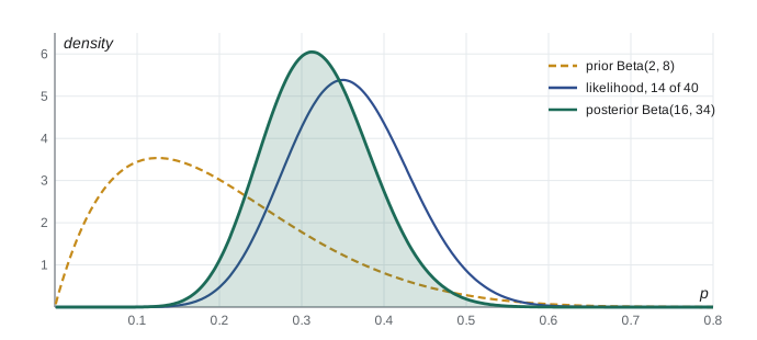
A new treatment is tried on 40 patients and 14 respond. Earlier studies of similar treatments suggest a response rate around 20%, encoded as a Beta(2, 8) prior. Find the posterior, a 95% credible interval, and the posterior probability that the response rate exceeds 25%.
Show solution
- The posterior is Beta\((2 + 14, 8 + 26)\) = Beta(16, 34).
- Its mean is \(16/50 = 0.32\), between the prior mean 0.20 and the sample proportion 0.35, closer to the data because the prior is worth only 10 observations.
- The 2.5% and 97.5% points of Beta(16, 34), found numerically, are about 0.200 and 0.454.
- Integrating the posterior density above 0.25 gives \(P(p > 0.25 \mid x) \approx 0.86\).
Answer: Posterior Beta(16, 34), mean 0.32, 95% credible interval 0.20 to 0.45, and an 86% posterior probability that the response rate exceeds 25%. A frequentist analysis gives a 95% Wilson confidence interval of 0.22 to 0.51.
Credible intervals and confidence intervals
A 95% credible interval \([l, u]\) satisfies \(P(l \le \theta \le u \mid x) = 0.95\). It supports exactly the statement that lesson 8 warned cannot be made about a confidence interval: given the data and the prior, the probability that \(\theta\) lies in the interval is 0.95. The price is the prior, which must be specified and defended. The equal-tailed interval puts 2.5% of posterior probability in each tail; the highest posterior density interval is the shortest interval with 95% probability.
In large samples the two approaches usually agree. The Bernstein–von Mises theorem states that, under regularity conditions and for any prior that is positive and continuous near the true value, the posterior is approximately normal with mean \(\hat\theta\) and variance \(1/(nI(\hat\theta))\). Credible intervals then coincide with Wald intervals to first order, and the prior's influence fades. With a flat Beta(1, 1) prior the trial's credible interval is about 0.22 to 0.51, almost identical to the Wilson interval. Differences matter when samples are small, when the prior is strong, or when there are many parameters.
Choosing a prior
Priors can encode genuine earlier evidence, as in the trial, or aim to be uninformative. A flat prior is not invariant: flat on \(p\) is not flat on the log-odds. Harold Jeffreys proposed in 1946 the prior \(\pi(\theta) \propto \sqrt{I(\theta)}\), built from the Fisher information, which gives the same answer under any reparameterization. For a binomial proportion it is Beta(1/2, 1/2). Whatever the choice, a responsible analysis checks the sensitivity of its conclusions to reasonable alternative priors.
Conjugate priors are convenient but limited. For realistic models the posterior's normalizing integral has no closed form, and modern Bayesian computation relies on Markov chain Monte Carlo, which draws a dependent sample from the posterior without computing the integral. The Metropolis algorithm of 1953, generalized by W. K. Hastings in 1970, and the Gibbs sampler, popularized for statistics by Alan Gelfand and Adrian Smith in 1990, made Bayesian methods practical for complex models.
Capstone: a full likelihood analysis
A manufacturer tests 30 electronic modules until failure and records their lifetimes in hours. The aim is to estimate the mean lifetime with an honest measure of uncertainty and to decide whether the simple exponential model, which implies a constant failure rate with no wear-out, is adequate. The analysis follows the course step by step.
Step 1, model. The exponential with rate \(\lambda\) is the natural first model, with sufficient statistic \(\sum t_i\) (lesson 7). The gamma with shape \(\alpha\) and rate \(\beta\) contains it as the case \(\alpha = 1\); a shape above 1 means a failure rate that increases with age.
Step 2, estimation. The exponential MLE is \(\hat\lambda = 1/\bar t\) (lesson 5). For the gamma, the moment estimate starts Newton's method on \(\log\alpha - \psi(\alpha) = \log\bar t - \overline{\log t}\), and then \(\hat\beta = \hat\alpha/\bar t\) (lessons 4 and 5).
Step 3, uncertainty. The standard error of \(\hat\alpha\), accounting for the estimated rate, is the corresponding diagonal entry of the inverse information matrix, which simplifies to \(\sqrt{\alpha/(n[\alpha\psi'(\alpha) - 1])}\) (lesson 6). The MLE of the mean \(\alpha/\beta\) is \(\bar t\) in both models, but its standard error differs: \(\bar t/\sqrt{n\alpha}\) under the gamma and \(\bar t/\sqrt n\) under the exponential.
Step 4, testing. The likelihood ratio statistic \(G = 2[\ell_{\text{gamma}} - \ell_{\text{exp}}]\) tests \(\alpha = 1\), with one degree of freedom by Wilks's theorem (lesson 10). The null value is in the interior of the parameter space, so no boundary correction is needed. AIC gives a second view.
import math, random
from statistics import mean

def beta_pdf(p, a, b):
    return math.exp((a - 1) * math.log(p) + (b - 1) * math.log(1 - p)
                    + math.lgamma(a + b) - math.lgamma(a) - math.lgamma(b))
def beta_quantile(q, a, b, m=20000):
    acc = 0.0
    for i in range(1, m):
        p = i / m; acc += beta_pdf(p, a, b) / m
        if acc >= q: return p
    return 1.0

# clinical trial: prior Beta(2, 8), 14 responders out of 40
a0, b0, k, n = 2, 8, 14, 40
a1, b1 = a0 + k, b0 + n - k
print(f"posterior Beta({a1}, {b1}): mean {a1 / (a1 + b1):.3f}, MLE {k / n:.3f}, prior mean {a0 / (a0 + b0):.3f}")
lo, hi = beta_quantile(0.025, a1, b1), beta_quantile(0.975, a1, b1)
print(f"95% credible interval {lo:.3f} to {hi:.3f}")
above = sum(beta_pdf(i / 20000, a1, b1) for i in range(int(0.25 * 20000), 20000)) / 20000
print(f"posterior P(p > 0.25) = {above:.3f}")
z = 1.96; ph = k / n
c = (ph + z * z / (2 * n)) / (1 + z * z / n)
h = z * math.sqrt(ph * (1 - ph) / n + z * z / (4 * n * n)) / (1 + z * z / n)
print(f"Wilson 95% confidence interval {c - h:.3f} to {c + h:.3f}")
# flat prior for comparison
print(f"flat prior Beta(1,1): interval {beta_quantile(0.025, 15, 27):.3f} to {beta_quantile(0.975, 15, 27):.3f}")

# capstone: a full likelihood analysis of 30 failure times (hours)
rng = random.Random(12)
t = sorted(round(rng.gammavariate(1.8, 250), 1) for _ in range(30))
print("data summary: n", len(t), "mean", round(mean(t), 1), "min", t[0], "max", t[-1])
def digamma(a):
    r = 0.0
    while a < 6: r -= 1 / a; a += 1
    f = 1 / (a * a)
    return r + math.log(a) - 0.5 / a - f * (1 / 12 - f * (1 / 120 - f / 252))
def trigamma(a, h=1e-5): return (digamma(a + h) - digamma(a - h)) / (2 * h)
m = mean(t); s = math.log(m) - mean(math.log(v) for v in t)
a = 0.5 / s
for _ in range(20): a -= (math.log(a) - digamma(a) - s) / (1 / a - trigamma(a))
rate = a / m
ll_gamma = sum(a * math.log(rate) - math.lgamma(a) + (a - 1) * math.log(v) - rate * v for v in t)
ll_exp = sum(math.log(1 / m) - v / m for v in t)
G = 2 * (ll_gamma - ll_exp)
from statistics import NormalDist
pv = 2 * (1 - NormalDist().cdf(math.sqrt(G)))
n = len(t)
se_a = math.sqrt(a / (n * (a * trigamma(a) - 1)))
print(f"exponential: mean {m:.1f}, loglik {ll_exp:.2f}")
print(f"gamma: shape {a:.3f} (se {se_a:.3f}), rate {rate:.5f}, loglik {ll_gamma:.2f}")
print(f"LR test of shape = 1: G = {G:.2f}, p = {pv:.4f}; AIC exp {-2*ll_exp+2:.1f}, gamma {-2*ll_gamma+4:.1f}")
print(f"mean life {m:.1f} h: se {m / math.sqrt(n * a):.1f} under the gamma, {m / math.sqrt(n):.1f} under the exponential")
print(f"Wald test of shape = 1: z = {(a - 1) / se_a:.2f}")posterior Beta(16, 34): mean 0.320, MLE 0.350, prior mean 0.200 95% credible interval 0.200 to 0.454 posterior P(p > 0.25) = 0.858 Wilson 95% confidence interval 0.221 to 0.505 flat prior Beta(1,1): interval 0.221 to 0.506 data summary: n 30 mean 356.1 min 27.4 max 1106.5 exponential: mean 356.1, loglik -206.25 gamma: shape 1.697 (se 0.402), rate 0.00477, loglik -204.09 LR test of shape = 1: G = 4.32, p = 0.0377; AIC exp 414.5, gamma 412.2 mean life 356.1 h: se 49.9 under the gamma, 65.0 under the exponential Wald test of shape = 1: z = 1.73
Step 5, report. The trial results reproduce the worked example. For the modules, the gamma shape estimate is about 1.7, the likelihood ratio statistic is about 4.3 with a p-value near 0.04, and the gamma has the lower AIC: there is moderate evidence of wear-out, and the exponential model is doubtful. The choice matters for the reported precision. The mean lifetime estimate is about 356 hours either way, but its standard error is about 50 hours under the gamma and 65 hours under the exponential, which ignores the data's smaller relative spread. The Wald test of \(\alpha = 1\) gives \(z \approx 1.73\), a two-sided p-value near 0.08, which is weaker than the likelihood ratio test: in a sample of 30, the members of the trinity can disagree, and the likelihood ratio, which respects the skewed shape of the log-likelihood, is the one to trust. A final report would state the model, the estimates with standard errors or intervals, the test of the exponential model, and a plot of the fitted density over a histogram of the data, followed by checks against fresh data as they arrive.
Looking back
The course has followed one idea through many forms. Data are modelled as draws from a distribution with unknown parameters; the likelihood says how well each parameter value explains the data; and its peak, curvature and ratios give estimates, standard errors, intervals and tests. Sufficiency explains why the likelihood captures everything the data say about the parameter; the Cramér–Rao bound and asymptotic efficiency explain why the MLE is hard to beat; the Neyman–Pearson lemma and Wilks's theorem make likelihood ratios the basis of testing; least squares is the likelihood solution for normal linear models; and Bayesian inference turns the same likelihood into a posterior. Beyond this course lie generalized linear models, mixed models, nonparametric and robust methods, and the high-dimensional problems of modern data science, all built on these foundations.
Common mistakes
MistakeTreating the prior as a technicality.
InsteadA strong prior can dominate a small sample; report the prior and check how sensitive conclusions are to it.
MistakeAssuming a flat prior is uninformative on every scale.
InsteadFlat on one parameterization is not flat on another; Jeffreys’s prior is invariant.
MistakeCalling a credible interval a confidence interval.
InsteadThey answer different questions, though in large samples with weak priors they are numerically close.
MistakeReporting a standard error from a model rejected by the data.
InsteadThe exponential standard error for the mean lifetime is too large here because the model is wrong.
MistakeRelying on the Wald test in small samples.
InsteadThe likelihood ratio test is usually more reliable, as the gamma shape test shows.
Summary and key terms
- Bayesian inference: posterior \(\propto\) likelihood \(\times\) prior.
- The beta prior is conjugate to the binomial: Beta\((a, b)\) becomes Beta\((a + x, b + n - x)\).
- The posterior mean is a weighted average of the prior mean and the MLE, with weight on the data growing with n.
- A credible interval has a direct probability interpretation given the prior; Bernstein–von Mises links it to confidence intervals in large samples.
- Jeffreys’s prior is proportional to the square root of the Fisher information.
- A full analysis chooses a model, estimates by maximum likelihood, quantifies uncertainty, tests simpler models and reports clearly.
- prior distribution
- The distribution expressing beliefs about a parameter before seeing the data.
- posterior distribution
- The conditional distribution of the parameter given the data.
- conjugate prior
- A prior family for which the posterior is in the same family.
- credible interval
- An interval containing a stated posterior probability.
- Jeffreys prior
- \(\pi(\theta) \propto \sqrt{I(\theta)}\).
- Bernstein–von Mises theorem
- In large samples, the posterior is approximately normal around the MLE.
- Markov chain Monte Carlo
- Simulation methods that sample from a posterior without computing its normalizing constant.
Practice problems
Work each problem on paper first, then reveal the answer to check.
With a Beta(1, 1) prior and 7 successes in 10 trials, what is the posterior and its mean?
Show answer
Beta(8, 4), mean \(8/12 \approx 0.667\).
A Poisson rate has a Gamma(3, 1) prior (shape 3, rate 1). Counts over 5 days total 18. Find the posterior mean.
Show answer
Gamma\((3 + 18, 1 + 5)\) = Gamma(21, 6), mean 3.5.
Show that the posterior mean of a beta-binomial model tends to \(x/n\) as \(n\) grows with \(x/n\) fixed.
Show answer
The weight \(n/(a + b + n) \to 1\).
Find the Jeffreys prior for a Poisson mean.
Show answer
\(I(\lambda) = 1/\lambda\), so \(\pi(\lambda) \propto \lambda^{-1/2}\).
In the capstone, why does the gamma model give a smaller standard error for the mean lifetime?
Show answer
The standard error is \(\bar t/\sqrt{n\alpha}\), and \(\hat\alpha > 1\) means the lifetimes are less variable relative to their mean than exponential lifetimes would be.
A gamma fit and an exponential fit have log-likelihoods \(-310.4\) and \(-312.9\). Compute G and the AIC values.
Show answer
\(G = 5.0\) on 1 df (p about 0.025); AIC 624.8 for gamma (2 parameters) and 627.8 for exponential (1 parameter).
Lesson quiz · 5 questions
Score 60% or more to complete this lesson.
Create a free account to save your progress, take quizzes and earn a certificate.