Sufficiency, the Rao–Blackwell theorem and the Cramér–Rao bound

Lessons 3 to 6 compared estimators by their bias, variance and mean squared error. This lesson asks two deeper questions. First, how much of the data does an estimator really need? Often a single summary, such as the total of a Poisson sample, carries all the information about the parameter, and the rest of the data can be discarded without loss. Second, how small can the variance of an unbiased estimator be? The Cramér–Rao inequality gives a lower bound, and the Rao–Blackwell and Lehmann–Scheffé theorems show how to find the unbiased estimator that achieves the smallest variance possible. Fisher introduced sufficiency in his 1922 paper. C. R. Rao proved both the variance bound and the improvement theorem in a single 1945 paper, written in his mid-twenties; Harald Cramér gave the bound in his 1946 book, and David Blackwell published the improvement theorem independently in 1947.

Sufficient statistics

A statistic \(T = T(X_1, \ldots, X_n)\) is sufficient for \(\theta\) if the conditional distribution of the sample given \(T\) does not depend on \(\theta\). Once \(T\) is known, the rest of the data is like the outcome of a random device with known probabilities, and so it cannot tell us anything more about \(\theta\).

Bernoulli trials give the standard example. Let \(X_1, \ldots, X_n\) be iid Bernoulli(\(p\)) and \(T = \sum X_i\). For any sequence \(x\) with \(t\) ones,

Given the number of successes, every arrangement is equally likely, whatever \(p\) is. The order in which successes occurred carries no information about \(p\), and \(T\) is sufficient.

The factorization theorem

Checking the definition directly is tedious. The factorization theorem, due to Fisher and stated in general form by Neyman in 1935, gives an easy test: \(T\) is sufficient for \(\theta\) if and only if the joint density or pmf can be written as

where \(g\) depends on the data only through \(T(x)\) and \(h\) does not involve \(\theta\). Paul Halmos and Leonard Savage extended the theorem to general dominated families in 1949. Examples follow at once.

Poisson: \(f(x; \lambda) = \lambda^{\sum x_i}e^{-n\lambda}/\prod x_i!\), so \(\sum X_i\) is sufficient. Exponential: \(\lambda^n e^{-\lambda\sum x_i}\), so \(\sum X_i\) is sufficient. Normal with both parameters unknown: the density is a function of \(\sum x_i\) and \(\sum x_i^2\), so the pair \((\bar X, S^2)\) is sufficient. Uniform on \([0, \theta]\): \(\theta^{-n}\mathbf{1}\{x_{(n)} \le \theta\}\mathbf{1}\{x_{(1)} \ge 0\}\), so the maximum \(X_{(n)}\) is sufficient.

All but the last are members of the exponential family, whose densities have the form \(h(x)\exp\{\eta(\theta)T(x) - A(\theta)\}\). For an iid sample from such a family, \(\sum T(X_i)\) is sufficient, and its dimension stays fixed as \(n\) grows. The Pitman–Koopman–Darmois theorem of 1935 and 1936 shows that, among families whose support does not depend on \(\theta\), only exponential families have a sufficient statistic of fixed dimension. For a Cauchy sample, by contrast, nothing short of the full set of order statistics is sufficient.

Minimal sufficiency

The whole sample is always sufficient, so sufficiency alone is not much of a reduction. A sufficient statistic is minimal if it is a function of every other sufficient statistic: it achieves the greatest possible data reduction. A practical criterion, due to Lehmann and Scheffé, is that \(T\) is minimal sufficient if the ratio \(f(x; \theta)/f(y; \theta)\) is free of \(\theta\) exactly when \(T(x) = T(y)\). For the Poisson the ratio is \(\lambda^{\sum x_i - \sum y_i}\) times a constant, which is free of \(\lambda\) exactly when the totals match, so \(\sum X_i\) is minimal sufficient. Note that a sufficient statistic is determined only up to one-to-one functions: \(\bar X\) is as good as \(\sum X_i\).

Sufficiency connects directly to the likelihood. By the factorization theorem, the likelihood depends on the data only through \(T\), so the MLE is always a function of a sufficient statistic, and two samples with the same value of a minimal sufficient statistic have proportional likelihood functions.

The Rao–Blackwell theorem

Suppose \(W\) is any unbiased estimator of \(\tau(\theta)\) and \(T\) is sufficient. Define \(W^* = E[W \mid T]\). Because \(T\) is sufficient, this conditional expectation does not depend on \(\theta\), so \(W^*\) is a genuine statistic. Then

The first equation is the tower property, and the second is the law of total variance. So conditioning on a sufficient statistic never hurts and usually helps: \(W^*\) is unbiased with variance no larger than \(W\), with equality only when \(W\) was already a function of \(T\). The theorem turns a crude unbiased estimator into a good one.

Completeness and the Lehmann–Scheffé theorem

Rao–Blackwell improves an estimator, but different starting points might lead to different improved estimators. Completeness rules this out. A statistic \(T\) is complete if \(E_\theta[g(T)] = 0\) for all \(\theta\) implies \(g(T) = 0\) with probability one: no non-trivial function of \(T\) has mean zero everywhere. The sufficient statistic \(\sum T(X_i)\) of a full-rank exponential family is complete, and so is the maximum of a uniform sample.

The Lehmann–Scheffé theorem of 1950 then says: if \(T\) is complete and sufficient, and \(W^*\) is an unbiased estimator that is a function of \(T\), then \(W^*\) is the unique uniformly minimum variance unbiased estimator (UMVUE) of its mean. If there were two unbiased functions of \(T\), their difference would have mean zero for all \(\theta\), so by completeness they are equal. This settles the examples: \((1 - 1/n)^{\sum X_i}\) is the UMVUE of \(e^{-\lambda}\), \(\bar X\) and \(S^2\) are the UMVUEs of the normal mean and variance, and \(\frac{n+1}{n}X_{(n)}\) is the UMVUE of the uniform endpoint.

Ancillary statistics and Basu's theorem

At the opposite extreme from a sufficient statistic is an ancillary one, whose distribution does not depend on \(\theta\) at all. For a normal sample with known variance and unknown mean, the sample variance \(S^2\) is ancillary: shifting every observation by the same amount leaves it unchanged. On its own an ancillary statistic says nothing about \(\theta\), yet Fisher argued that it can tell us how precise an estimate is, and that inference should be conditional on its observed value. A sample in which the observations happen to be widely spread gives a less informative mean than one in which they are tightly clustered.

Debabrata Basu proved a striking result in 1955: a complete sufficient statistic is independent of every ancillary statistic. Applied to the normal model with \(\sigma^2\) fixed, \(\bar X\) is complete and sufficient for \(\mu\) and \(S^2\) is ancillary, so \(\bar X\) and \(S^2\) are independent. Since \(\sigma^2\) was arbitrary, this gives a short proof of the independence used in lesson 2 to derive the \(t\) distribution. Basu's theorem is often the quickest way to show that two statistics are independent without computing a joint distribution.

The Cramér–Rao lower bound

How small can the variance of an unbiased estimator be? Let \(W\) be unbiased for \(\tau(\theta)\) and let \(U = \partial_\theta\log f(X; \theta)\) be the score of the whole sample, which has mean zero and variance \(nI(\theta)\) under the regularity conditions of lesson 6. Differentiating \(E_\theta[W] = \tau(\theta)\) under the integral sign gives \(\mathrm{Cov}(W, U) = \tau'(\theta)\). The Cauchy–Schwarz inequality \(\mathrm{Cov}(W, U)^2 \le \mathrm{Var}(W)\mathrm{Var}(U)\) then gives

For \(\tau(\theta) = \theta\) the bound is \(1/(nI(\theta))\), the asymptotic variance of the MLE from lesson 6. Equality in Cauchy–Schwarz holds only if \(W\) is a linear function of \(U\), which happens only in exponential families with \(W\) a linear function of the natural sufficient statistic. So the bound is attained in special cases and approached by the MLE asymptotically.

Examples. Poisson: \(\bar X\) has variance \(\lambda/n = 1/(nI)\), so it attains the bound. Normal variance: the bound for estimating \(\sigma^2\) is \(2\sigma^4/n\), while \(S^2\) has variance \(2\sigma^4/(n - 1)\). The bound is not attained, yet \(S^2\) is the UMVUE, so in this case no unbiased estimator reaches the bound. Estimating \(e^{-\lambda}\) for the Poisson: the bound is \(\lambda e^{-2\lambda}/n\), while the UMVUE has variance \(e^{-2\lambda}(e^{\lambda/n} - 1)\), slightly larger.

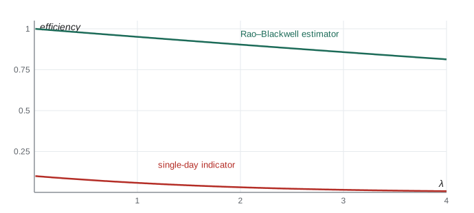
The figure shows how large the gain from conditioning is. With 10 days, the single-day indicator has efficiency \(\lambda/[n(e^\lambda - 1)]\), which never exceeds \(1/n = 0.1\) and falls towards zero as \(\lambda\) grows, while the improved estimator stays above 0.8 throughout. At \(\lambda = 2\) its efficiency is \(0.2/(e^{0.2} - 1) \approx 0.90\).

When the bound does not apply

The Cramér–Rao argument needs differentiation under the integral sign, which fails when the support depends on \(\theta\). For the uniform on \([0, \theta]\), the formal information \(E[(\partial_\theta\log f)^2] = 1/\theta^2\) would give a bound of \(\theta^2/n\), yet the UMVUE \(\frac{n+1}{n}X_{(n)}\) has variance \(\theta^2/[n(n + 2)]\), smaller by a factor of about \(n\). There is no contradiction: the bound simply does not hold here. Such non-regular models allow estimation at rate \(1/n\) rather than \(1/\sqrt n\), which is why the sample maximum is so effective.

import math, random
from statistics import mean, pvariance

rng = random.Random(7)
def poisson(lam):
    k, p, L = 0, 1.0, math.exp(-lam)
    while True:
        p *= rng.random()
        if p < L: return k
        k += 1

lam, n, reps = 2.0, 10, 20000
crude, rb, mle = [], [], []
for _ in range(reps):
    x = [poisson(lam) for _ in range(n)]
    t = sum(x)
    crude.append(1.0 if x[0] == 0 else 0.0)
    rb.append((1 - 1 / n) ** t)
    mle.append(math.exp(-t / n))
target = math.exp(-lam)
bound = lam * math.exp(-2 * lam) / n
print(f"target e^-2 = {target:.5f}, Cramer-Rao bound {bound:.6f}")
for name, est in (("crude", crude), ("Rao-Blackwell", rb), ("MLE", mle)):
    print(f"{name:14s} mean {mean(est):.5f}  var {pvariance(est):.6f}")
print(f"exact UMVUE variance {math.exp(-2 * lam) * (math.exp(lam / n) - 1):.6f}")

# uniform: the 'bound' theta^2/n does not apply
theta, n = 10.0, 20
u = [(n + 1) / n * max(rng.uniform(0, theta) for _ in range(n)) for _ in range(20000)]
print(f"uniform UMVUE var {pvariance(u):.4f}, theory {theta**2 / (n * (n + 2)):.4f}, "
      f"formal 'bound' {theta**2 / n:.4f}")

target e^-2 = 0.13534, Cramer-Rao bound 0.003663
crude          mean 0.13770  var 0.118739
Rao-Blackwell  mean 0.13515  var 0.003995
MLE            mean 0.14890  var 0.004351
exact UMVUE variance 0.004055
uniform UMVUE var 0.2237, theory 0.2273, formal 'bound' 5.0000

The simulation confirms the theory. All three estimators are close to \(e^{-2} \approx 0.135\) on average, though the MLE is slightly biased upward. The crude indicator has a variance many times larger than the bound; the Rao–Blackwell estimator has a variance just above the bound and close to the exact formula. The MLE has a variance comparable to the UMVUE's here, but it pays for its bias, which a mean squared error comparison would include. For the uniform, the variance of the UMVUE is far below the formal bound, confirming that the inequality does not hold for non-regular models.