Maximum likelihood estimation

Maximum likelihood is the most widely used method of estimation in statistics. Its principle is simple: among all parameter values, choose the one that makes the observed data most probable. Ronald Fisher proposed it in 1912 as a student and developed it in his great paper of 1922, which also introduced sufficiency, efficiency and consistency as criteria. The method applies to almost any parametric model, gives estimators that are functions of sufficient statistics, behaves well under reparameterization, and, as lesson 6 shows, is asymptotically optimal under regularity conditions. It also gives the likelihood function, which is the basis of likelihood ratio tests (lesson 10) and of Bayesian inference (lesson 12).

The likelihood function

Let the data \(x = (x_1, \ldots, x_n)\) have joint pmf or density \(f(x; \theta)\). Regarded as a function of \(\theta\) with the data held fixed, it is called the likelihood function, \(L(\theta) = f(x; \theta)\). For an iid sample,

The log-likelihood \(\ell\) is easier to work with because it turns a product into a sum, and taking logs does not move the maximum. The likelihood is not a probability distribution over \(\theta\): it need not integrate to one, and only ratios \(L(\theta_1)/L(\theta_2)\) carry meaning. A likelihood ratio of 10 says that the observed data were ten times as probable under \(\theta_1\) as under \(\theta_2\). Constant factors that do not involve \(\theta\) can be dropped, which is why the binomial coefficient never matters when estimating \(p\).

The maximum likelihood estimator (MLE) \(\hat\theta\) is the value of \(\theta\) that maximizes \(L(\theta)\) over \(\Theta\). When \(\ell\) is differentiable and the maximum is in the interior of \(\Theta\), it solves the likelihood equation \(\ell'(\theta) = 0\). The derivative \(U(\theta) = \ell'(\theta)\) is called the score. One must then check that the solution is a maximum, not a minimum or saddle point, and that it is the global maximum, not a local one. For the standard examples \(\ell\) is concave and the solution is unique.

Standard examples

Bernoulli. With \(x\) successes in \(n\) trials, \(\ell(p) = x\log p + (n - x)\log(1 - p)\). The score is \(x/p - (n - x)/(1 - p)\), which is zero at \(\hat p = x/n\), the sample proportion. The second derivative \(-x/p^2 - (n-x)/(1-p)^2\) is negative, so this is the maximum. If \(x = 0\), the likelihood \((1 - p)^n\) is decreasing and the MLE is the boundary value \(\hat p = 0\), found by inspection, not by setting a derivative to zero.

Poisson. \(\ell(\lambda) = \sum x_i\log\lambda - n\lambda - \sum\log x_i!\), with score \(\sum x_i/\lambda - n\), so \(\hat\lambda = \bar x\). Exponential with rate \(\lambda\). \(\ell(\lambda) = n\log\lambda - \lambda\sum x_i\), so \(\hat\lambda = 1/\bar x\), the same as the moment estimator.

Normal with both parameters unknown. The log-likelihood is

Setting the partial derivative in \(\mu\) to zero gives \(\sum(x_i - \mu) = 0\), so \(\hat\mu = \bar x\) whatever \(\sigma^2\) is. Substituting and differentiating in \(\sigma^2\) gives \(-n/(2\sigma^2) + \sum(x_i - \bar x)^2/(2\sigma^4) = 0\), so \(\hat\sigma^2 = \frac1n\sum(x_i - \bar x)^2\). The MLE of the variance divides by \(n\), not \(n - 1\): maximum likelihood estimators need not be unbiased. As lesson 3 showed, \(\hat\sigma^2\) actually has smaller mean squared error than \(S^2\) for normal data.

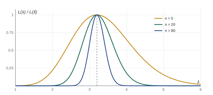
The curvature of the log-likelihood at its peak measures how much the data say about \(\theta\). A sharply curved log-likelihood rules out all but a narrow range of values; a flat one leaves many values almost equally supported. For the Poisson, \(\ell''(\hat\lambda) = -n/\hat\lambda\), which grows in magnitude with \(n\). Lesson 6 makes this precise: the inverse of the curvature, called the observed information, estimates the variance of the MLE.

A boundary case: the uniform

For an iid sample from the uniform on \([0, \theta]\), the density of each observation is \(1/\theta\) on \([0, \theta]\) and zero elsewhere, so

The likelihood is zero for \(\theta\) below the sample maximum and decreasing above it, so the MLE is \(\hat\theta = x_{(n)}\). The likelihood equation has no solution here, since the maximum is at a point where \(L\) jumps. The MLE is biased, with \(E[X_{(n)}] = n\theta/(n + 1)\), but it is a function of the sufficient statistic, and the bias-corrected version \(\frac{n+1}{n}X_{(n)}\) is the best unbiased estimator. This example breaks the regularity conditions of lesson 6, because the support depends on \(\theta\).

Invariance

If \(\hat\theta\) is the MLE of \(\theta\), then for any function \(g\), the MLE of \(g(\theta)\) is \(g(\hat\theta)\). For one-to-one \(g\) this is immediate: reparameterizing does not change which distribution makes the data most probable. For general \(g\), the invariance property holds when the likelihood of \(\eta = g(\theta)\) is defined as the maximum of \(L(\theta)\) over \(\{\theta : g(\theta) = \eta\}\), the profile likelihood. So the MLE of the normal standard deviation is \(\hat\sigma = \sqrt{\hat\sigma^2}\), the MLE of the probability that an exponential lifetime exceeds 10 years is \(e^{-10\hat\lambda}\), and the MLE of the odds \(p/(1 - p)\) is \(\hat p/(1 - \hat p)\). Unbiasedness has no such property, which is one of the reasons the likelihood approach is preferred.

The example shows one of the great strengths of the likelihood approach. Incomplete observations such as censored lifetimes, which have no natural place in a method of moments, enter the likelihood through their probability. Survival analysis in medicine and reliability analysis in engineering are built on this idea.

Numerical maximization

For most realistic models the likelihood equation has no closed-form solution, and the MLE is found numerically. Newton's method iterates

which converges quadratically near the maximum when \(\ell''\) is negative there. Fisher scoring replaces \(-\ell''(\theta_k)\) with its expected value, the Fisher information \(nI(\theta_k)\) of lesson 6, which is often simpler and more stable. For several parameters, the derivative becomes the gradient and the second derivative the Hessian matrix. Good starting values matter, and the method of moments supplies them. For the gamma distribution, the likelihood equations reduce to one equation in the shape \(\alpha\): \(\log\alpha - \psi(\alpha) = \log\bar x - \overline{\log x}\), where \(\psi\) is the digamma function, and then \(\hat\beta = \hat\alpha/\bar x\). The right side is positive by Jensen's inequality, and Newton's method solves the equation in a few steps.

import math, random
from statistics import mean

rng = random.Random(252)

# Poisson: grid search versus closed form
x = [rng.choice([1, 2, 3, 3, 4, 4, 5, 6]) for _ in range(20)]
ll = lambda lam: sum(xi * math.log(lam) - lam - math.lgamma(xi + 1) for xi in x)
grid = [i / 1000 for i in range(1000, 8000)]
best = max(grid, key=ll)
print(f"Poisson: grid MLE {best:.3f}, sample mean {mean(x):.3f}")

# censored exponential lifetimes (pump test)
d, T = 7, 3150 + 3 * 1000
print(f"censored exponential: lambda-hat {d / T:.6f} per hour, mean life {T / d:.1f} hours")

# gamma: Newton's method for the shape, from a moment starting value
def digamma(a):
    r = 0.0
    while a < 6:
        r -= 1 / a; a += 1
    f = 1 / (a * a)
    return r + math.log(a) - 0.5 / a - f * (1 / 12 - f * (1 / 120 - f / 252))
def trigamma(a, h=1e-5):
    return (digamma(a + h) - digamma(a - h)) / (2 * h)
y = [rng.gammavariate(2.5, 1 / 0.5) for _ in range(150)]
m = mean(y); s = math.log(m) - mean(math.log(v) for v in y)
a = m * m / (sum((v - m) ** 2 for v in y) / len(y))      # moment estimate
print(f"gamma: moment start alpha = {a:.4f}")
for k in range(6):
    g = math.log(a) - digamma(a) - s
    a -= g / (1 / a - trigamma(a))
    print(f"  Newton step {k + 1}: alpha = {a:.6f}")
print(f"gamma MLE: alpha-hat {a:.4f}, beta-hat {a / m:.4f}   (true 2.5, 0.5)")

# normal: MLE of sigma^2 divides by n
z = [rng.gauss(50, 8) for _ in range(12)]
mz = mean(z); ss = sum((v - mz) ** 2 for v in z)
print(f"normal: mu-hat {mz:.3f}, sigma2-hat (MLE) {ss / len(z):.3f}, S^2 {ss / (len(z) - 1):.3f}")

Poisson: grid MLE 3.350, sample mean 3.350
censored exponential: lambda-hat 0.001138 per hour, mean life 878.6 hours
gamma: moment start alpha = 2.4927
  Newton step 1: alpha = 2.597420
  Newton step 2: alpha = 2.602262
  Newton step 3: alpha = 2.602272
  Newton step 4: alpha = 2.602272
  Newton step 5: alpha = 2.602272
  Newton step 6: alpha = 2.602272
gamma MLE: alpha-hat 2.6023, beta-hat 0.5374   (true 2.5, 0.5)
normal: mu-hat 50.022, sigma2-hat (MLE) 74.299, S^2 81.053

Newton's method for the gamma shape settles to six decimal places within a few steps from the moment estimate, as quadratic convergence predicts. The grid search for the Poisson agrees with the sample mean to the resolution of the grid. In practice software uses the same ideas with safeguards: step halving when the likelihood does not increase, parameter transformations to keep estimates inside \(\Theta\), and several starting points when the likelihood may have more than one peak.

When maximum likelihood misbehaves

The method is not foolproof. The likelihood may be unbounded: for a mixture of two normal distributions with unequal unknown variances, placing one component's mean at a data point and letting its variance shrink to zero sends the likelihood to infinity, so the global maximum is a useless degenerate solution and the sensible estimate is a local maximum. The MLE may not be unique, or may not exist, as in logistic regression with perfectly separated data. And when the number of parameters grows with the sample size, the MLE can be inconsistent: in the Neyman–Scott problem, pairs of observations share their own means \(\mu_i\) and a common variance \(\sigma^2\), and the MLE of \(\sigma^2\) converges to \(\sigma^2/2\). These are exceptions, but they are reminders that maximizing a function is a computation, and its answer must still make statistical sense.

A flat ridge: the binomial with unknown n

Lesson 4 showed that moment estimates of both \(n\) and \(p\) in a binomial model are unstable. The likelihood explains why. For counts \(x_1, \ldots, x_k\) from a binomial with both parameters unknown, the likelihood surface has a long, nearly flat ridge along which \(np\) stays close to \(\bar x\): a large \(n\) with a small \(p\) fits the data almost as well as a small \(n\) with a large \(p\). The MLE of \(n\) exists, but the log-likelihood changes by only a fraction of a unit over a wide range of \(n\), so the data barely distinguish those values. A flat likelihood is an honest report that the data carry little information, and no clever estimator can recover what is not there. The remedy is outside information: a known upper bound on \(n\), a second kind of data, or a prior distribution as in lesson 12.