
NUC-300 · Lesson 4 of 12 · 24 min
The diffusion equation
The core-follow code that produced last week's flux map solves a version of the neutron diffusion equation in three dimensions with two energy groups. Teodora wants Hana to derive the equation herself, solve it for the simplest possible case, and then write a small finite-difference solver so that the code stops being a black box. The derivation is short; its assumptions are where the physics lies.
A neutron balance in a small volume
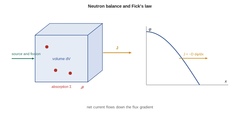
Consider a small volume in the reactor. The number of neutrons inside changes because of production by sources and fission, loss by absorption and net flow out through the surface. Written per unit volume for one energy group, this balance is the neutron continuity equation:
The left side is the rate of change of neutron density \(n = \phi/v\). The source term \(S\) includes fission, \(\nu \Sigma_f \phi\) in a multiplying medium, and any external source. The term \(\nabla \cdot \mathbf{J}\) is the net leakage out of the volume per unit volume. The equation is exact; the difficulty is that it has two unknowns, the flux and the current. Diffusion theory closes it with an approximate relation between them.
Fick's law
Where the flux varies in space, more neutrons scatter out of the high-flux side than the low-flux side, so a net current flows down the gradient. When scattering dominates absorption, the flux varies slowly over a mean free path, and the medium is far from boundaries, this gives Fick's law:
The diffusion coefficient \(D\), in centimetres, is one third of the transport mean free path. The transport cross section \(\Sigma_{tr}\) corrects the total cross section for the forward bias of scattering: light nuclei such as hydrogen scatter neutrons preferentially forward, with average cosine \(\bar{\mu}_0 = 2/(3A)\), so a neutron keeps more of its original direction and diffuses further. Heat conduction, chemical diffusion and neutron diffusion all share this mathematical form, which is why their solutions look alike.
The one-group diffusion equation
Substituting Fick's law into the continuity equation gives the time-dependent one-group diffusion equation. For steady state, the left side vanishes:
Divide by \(D\) and define the diffusion length \(L\), with \(L^2 = D/\Sigma_a\), the diffusion area. In a non-multiplying medium with source \(S\),
The diffusion area has a physical meaning: \(L^2\) is one sixth of the mean square straight-line distance a thermal neutron travels from where it becomes thermal to where it is absorbed. Light water has \(L \approx 2.8\) cm, graphite about 54 cm and pure heavy water more than 100 cm. Small \(L\) means thermal neutrons are absorbed close to where they appear; large \(L\) means they wander far, and leakage from a small core is larger.
| Moderator | D (cm) | Σ_a (cm⁻¹) | L (cm) |
|---|---|---|---|
| Light water | 0.16 | 0.0197 | about 2.8 |
| Heavy water (pure) | 0.87 | about 3 × 10⁻⁵ | over 100 |
| Graphite | 0.84 | 0.00027 | about 54 |
| Beryllium | 0.50 | 0.0012 | about 21 |
Boundary conditions
Physical solutions must satisfy a few conditions. The flux is finite and non-negative everywhere it represents real neutrons. At an interface between two materials, the flux and the normal component of the current are continuous. At a free surface facing vacuum, no neutrons return, which in diffusion theory is approximated by requiring the flux to extrapolate linearly to zero a short distance beyond the surface. The extrapolation distance is
For large power cores \(d\) is a few centimetres and often negligible, but for small research cores and for thin regions it matters. Diffusion theory is least accurate within a few mean free paths of boundaries, strong absorbers and sources, where the angular distribution of neutrons is far from the near-isotropic picture Fick's law assumes. Transport theory, discussed in Reactor Physics II, handles those regions.
A first solution: a slab with a uniform source
Consider an infinite slab of non-multiplying material of half-thickness \(a\), with a uniform source \(S\) throughout and vacuum outside. Symmetry about \(x = 0\) gives \(d\phi/dx = 0\) there, and the flux vanishes at the extrapolated boundary \(x = a\) (here \(a\) already includes \(d\)). The solution is
Deep inside a thick slab, the flux reaches the infinite-medium value \(S/\Sigma_a\), at which absorption exactly balances the source. Within a few diffusion lengths of the surface it falls toward zero, because neutrons born there are likely to escape. The solution is a template for every leakage effect in this course: leakage is concentrated where the flux has curvature, and its importance depends on the size of the region compared with the diffusion length.
Solving the equation numerically
Real cores are not uniform, so the equation is solved numerically. Divide the slab into \(N\) intervals of width \(h\) and replace the second derivative with a central difference:
Each node gives one linear equation in its own flux and its two neighbours', so the whole problem becomes a tridiagonal matrix equation. The symmetry condition at the centre is handled by a mirror node, \(\phi_{-1} = \phi_1\), and the vacuum condition by \(\phi_N = 0\). Tridiagonal systems are solved directly, without iteration, by the Thomas algorithm, a streamlined form of Gaussian elimination.
Worked problem
Checking the solver
A slab of half-width 100 cm has \(D = 0.9\) cm, \(\Sigma_a = 0.02\ \text{cm}^{-1}\) and \(S = 10^8\) neutrons per cm³ per second. Find \(L\) and the flux at the centre.
Show solution
- \(L = \sqrt{0.9/0.02} = 6.71\) cm.
- The slab is about fifteen diffusion lengths thick, so \(\cosh(0)/\cosh(100/6.71)\) is negligible at the centre.
- \(\phi(0) \approx S/\Sigma_a = 10^8/0.02 = 5.0 \times 10^9\ \text{cm}^{-2}\text{s}^{-1}\).
Answer: The centre is effectively an infinite medium; the flux only drops within a few diffusion lengths of the surface.
# One-group diffusion in a slab with a fixed source: finite differences vs exact.
import math
D, Sa, S = 0.9, 0.02, 1.0e8     # cm, 1/cm, n/cm3/s (non-multiplying medium, illustrative)
a = 100.0                        # half-width, cm (flux zero at extrapolated boundary)
L = math.sqrt(D / Sa)
N = 50; h = a / N
# unknowns phi_0..phi_{N-1}; symmetry at x=0, phi_N = 0
A = [list([0.0] * N) for _ in range(N)]; b = [S * h * h / D] * N
for i in range(N):
    A[i][i] = 2 + h * h / L ** 2
    if i > 0: A[i][i - 1] = -1
    if i < N - 1: A[i][i + 1] = -1
A[0][1] = -2   # mirror condition phi_-1 = phi_1
# tridiagonal solve (Thomas algorithm)
c = [0.0] * N; d = [0.0] * N
c[0] = A[0][1] / A[0][0]; d[0] = b[0] / A[0][0]
for i in range(1, N):
    m = A[i][i] - A[i][i - 1] * c[i - 1]
    c[i] = A[i][i + 1] / m if i < N - 1 else 0.0
    d[i] = (b[i] - A[i][i - 1] * d[i - 1]) / m
phi = [0.0] * N; phi[-1] = d[-1]
for i in range(N - 2, -1, -1): phi[i] = d[i] - c[i] * phi[i + 1]
exact = lambda x: S / Sa * (1 - math.cosh(x / L) / math.cosh(a / L))
print(f"diffusion length L = {L:.2f} cm")
for i in (0, 10, 25, 40, 49):
    x = i * h
print(f"x = {x:5.1f} cm numerical {phi[i]:.4e} exact {exact(x):.4e}")diffusion length L = 6.71 cm x = 0.0 cm numerical 5.0000e+09 exact 5.0000e+09 x = 20.0 cm numerical 5.0000e+09 exact 5.0000e+09 x = 50.0 cm numerical 4.9970e+09 exact 4.9971e+09 x = 80.0 cm numerical 4.7436e+09 exact 4.7464e+09 x = 98.0 cm numerical 1.2850e+09 exact 1.2890e+09
The numerical and exact results agree to better than half a percent even near the boundary with only 50 intervals, because each interval is a third of a diffusion length. With intervals much larger than \(L\), the finite-difference solution would lose accuracy where the flux curves sharply. A practical rule is that mesh spacing should be small compared with the diffusion length in each region, which is why light water reactor models need finer meshes than heavy water or graphite models.
What the diffusion length tells a designer
The diffusion length is more than a parameter; it is the natural ruler for every thermal neutron problem. A region much thinner than \(L\) is nearly transparent to diffusing neutrons, while a region several diffusion lengths thick behaves like an infinite medium in its interior. Flux disturbances, such as the dip near a control rod or the peak in a water gap, spread over a few diffusion lengths. Leakage from a core of size \(R\) scales roughly as \((L/R)^2\).
Teodora illustrates this with three numbers. In light water, \(L\) is under 3 cm, so a light water reactor's thermal flux responds very locally: an absorber pin depresses the flux in its own assembly and its neighbours but barely affects assemblies a metre away. In heavy water, \(L\) is more than a metre for the pure moderator, and still tens of centimetres in a CANDU lattice, so a disturbance in one part of the core is felt widely. In graphite, \(L\) of about half a metre explains why graphite-moderated cores are large.
The diffusion length also controls how fast a fixed source fills a non-multiplying region. In shielding and in the reflector problems of lesson 6, the flux from a source falls roughly as \(e^{-x/L}\) with distance, so a reflector several diffusion lengths thick returns almost every neutron that a thicker one would. This is the physical basis for the reflector savings that lesson 6 computes.
Worked problem
Flux from a plane source in water
In an infinite medium, the flux from a plane source falls as \(e^{-|x|/L}\). Using \(L = 2.8\) cm for water, find the fraction of the flux at the source plane that remains 10 cm away.
Show solution
- \(10/2.8 = 3.57\) diffusion lengths.
- \(e^{-3.57} = 0.028\).
Answer: Less than 3 percent remains, which is why a few tens of centimetres of water is an effective thermal neutron shield around a research reactor pool.
Two regions and interface conditions
Most real problems have more than one material. At the interface between a fuel region and a reflector, or between water and a steel structure, the flux and the current must both be continuous. The first condition says neutrons do not appear or vanish at the interface; the second says the net number crossing from one side equals the number arriving on the other. Because \(D\) differs between materials, the flux slope changes at the interface even though the flux and current are continuous: the slope is steeper on the side with smaller \(D\).
In a finite-difference solver, the interface conditions are built in automatically if the coefficients are written in conservative form, using an effective diffusion coefficient between neighbouring nodes such as the harmonic mean \(2D_iD_{i+1}/(D_i + D_{i+1})\). That small detail is what keeps a code's neutron balance exact across material boundaries. Hana adds it to her solver and checks that the total absorption plus leakage equals the total source to many decimal places, the same check every production code runs before reporting a result.
From diffusion to the reactor equation
In a multiplying medium the source is fission itself, \(S = \nu\Sigma_f \phi\), and the steady equation becomes homogeneous: every term is proportional to \(\phi\). Such an equation has a non-zero solution only for particular combinations of size and composition, the critical ones. Lesson 5 shows that writing the fission source as \(\nu\Sigma_f\phi/k\) turns the problem into an eigenvalue problem whose eigenvalue is \(k_{\text{eff}}\) and whose eigenfunction is the flux shape. The finite-difference solver built here becomes, with a power iteration added, a working criticality code.
Hana's mesh for a full CANDU core model would need far fewer points per metre than a light water model, because the heavy water lattice has long migration lengths. That is one reason the design codes used for the Darlington CANDU station could run on modest computers decades ago.
Common mistakes
MistakeApplying Fick's law right next to a vacuum boundary or strong absorber.
InsteadDiffusion is least accurate there; use the extrapolation distance or transport methods.
MistakeTreating D as the absorption mean free path.
InsteadD is one third of the transport mean free path.
MistakeUsing a mesh much coarser than the diffusion length.
InsteadKeep spacing small compared with L in each region.
MistakeForgetting current continuity at a material interface.
InsteadBoth φ and D dφ/dx are continuous across interfaces.
Summary and key terms
- The continuity equation balances production, absorption and leakage in each volume.
- Fick's law J = −D∇φ closes the balance, with D = 1/(3Σ_tr).
- Steady one-group diffusion: −D∇²φ + Σ_aφ = S, with diffusion area L² = D/Σ_a.
- Vacuum boundaries are modelled by extrapolating the flux to zero at d ≈ 2.13D.
- Finite differences turn the equation into a tridiagonal system solved by the Thomas algorithm.
- In a multiplying medium the equation becomes an eigenvalue problem for k_eff.
- Continuity equation
- The neutron balance: rate of change equals production minus absorption minus net leakage.
- Fick's law
- The approximation that net current is proportional to the negative gradient of flux.
- Diffusion coefficient
- D = 1/(3Σ_tr), one third of the transport mean free path.
- Diffusion length
- L = √(D/Σ_a); L² is one sixth of the mean square distance to absorption.
- Extrapolation distance
- The distance beyond a free surface at which the flux is extrapolated to zero, about 0.71 λ_tr.
- Transport cross section
- The total cross section corrected for forward scattering, Σ_t − μ̄₀Σ_s.
- Thomas algorithm
- A direct method for solving tridiagonal linear systems.
Practice problems
Work each problem on paper first, then reveal the answer to check.
Σ_tr = 0.4 cm⁻¹. Find D.
Show answer
D = 1/(3 × 0.4) = 0.83 cm.
D = 0.83 cm and Σ_a = 0.005 cm⁻¹. Find L.
Show answer
√(0.83/0.005) = 12.9 cm.
Find the extrapolation distance for D = 0.83 cm.
Show answer
2.13 × 0.83 = 1.8 cm.
In the slab example, why is the centre flux equal to S/Σ_a?
Show answer
The centre is many diffusion lengths from the surface, so leakage there is negligible.
Using the program, what is the numerical flux 2 cm inside the boundary?
Show answer
About 1.29 × 10⁹ cm⁻² s⁻¹.
What two quantities are continuous at a material interface?
Show answer
The flux and the normal current, −D dφ/dx.
Lesson quiz · 5 questions
Score 60% or more to complete this lesson.
Create a free account to save your progress, take quizzes and earn a certificate.