
MBA-502 · Lesson 11 of 12 · 25 min
The macro environment: growth, inflation, interest rates and exchange rates
The first ten lessons focused on microeconomics: decisions by individual firms, consumers and markets. But every firm also operates in a macroeconomic environment it cannot control. Recessions cut demand across industries; inflation raises input costs and changes how customers behave; interest rates determine the cost of capital and the value of long-lived investments; exchange rates move the competitiveness of exporters and the margins of importers; and trade policy can change the economics of a supply chain overnight. Managers do not need to forecast these variables better than professional economists, which is very hard, but they do need to understand how they work, how central banks respond, and how their own business is exposed. This lesson gives that understanding and shows how to build macro scenarios into plans.
Output, growth and the business cycle
Gross domestic product measures the market value of final goods and services produced in an economy in a period. It can be measured as the sum of spending, consumption plus investment plus government purchases plus net exports; as the sum of incomes, wages, profits, rents and interest; or as the sum of value added by each industry. Statistics Canada publishes GDP quarterly and monthly by industry. Real GDP adjusts for price changes and is the main measure of output; real GDP per person is a rough measure of living standards. Over long periods, real GDP grows because of more workers, more capital per worker and better technology and organization, which economists call total factor productivity. Canada's slow productivity growth relative to the United States since the 2000s has become a central policy concern.
In the short run, output fluctuates around its potential in the business cycle. Expansions are periods of rising output and employment; recessions are periods of falling output, usually identified in Canada by the C.D. Howe Institute's Business Cycle Council. The output gap, the difference between actual and potential output, is a key input to monetary policy: a positive gap tends to raise inflation, a negative gap to lower it. Unemployment rises in recessions and falls in expansions, as described by Okun's law, which links a percentage point of output gap to roughly half a percentage point of unemployment.
Industries differ greatly in their sensitivity to the cycle. Grace's grocery business is defensive: people keep eating in recessions, though they trade down to cheaper brands and private label. Daniel's automotive and industrial parts business is cyclical: vehicle and equipment purchases can be postponed, so Northfield's volumes fall sharply in downturns, and operating leverage, the high share of fixed costs discussed in Lesson 4, amplifies the effect on profit. Owen's energy business depends on commodity prices driven by the global cycle. Hana's health care demand is stable, but government budgets that fund it are cyclical. Kestrel's software sales depend on corporate budgets, which tighten in recessions, though tools that cut costs can sell well then. Knowing where a business sits helps managers plan capacity, inventory and financing.
Inflation
Inflation is a sustained rise in the general price level. Statistics Canada measures it with the consumer price index, which tracks the cost of a fixed basket of goods and services. The Bank of Canada targets 2 % inflation, the midpoint of a 1 % to 3 % control range, under an agreement with the federal government that is reviewed and renewed every five years. Inflation can be driven by demand, when spending outpaces the economy's capacity; by costs, when energy, food or wage shocks raise prices; and by expectations, when firms and workers build anticipated inflation into prices and wages. Expectations matter because they can make inflation self-sustaining, which is why central banks guard their credibility carefully.
Inflation surged in 2021 and 2022 as economies reopened, supply chains strained and energy prices spiked, peaking in Canada at 8.1 % in June 2022 before falling back toward the target by 2024. In 2026, energy prices rose again: in September 2026, Canadian consumer prices were 3.1 % higher than a year earlier, with gasoline up 27.8 %, while inflation excluding gasoline was a more moderate 2.2 %. Separating a temporary energy shock from broader inflation is exactly the judgment central banks must make.
For managers, inflation creates several challenges. Input costs rise at different rates, so margins shift between products. Customers become more price-sensitive and more likely to trade down. Contracts that are fixed in nominal terms lose real value for the seller, which is why long-term supply contracts often include indexation or escalation clauses. Wage negotiations become harder. And because accounting statements are in nominal terms, inflation can flatter reported profits through inventory gains and understate the cost of replacing assets. Daniel learned this in 2022, when Northfield's fixed-price contracts with some customers lost money as steel prices jumped; the company now includes steel surcharges indexed to a published price.
Real and nominal interest rates
The nominal interest rate i is what lenders quote; the real interest rate r is the return after inflation, and π^e is expected inflation. The Fisher equation, named after Irving Fisher, links them. Real rates matter for investment decisions: a 6 % loan with 4 % expected inflation is cheaper in real terms than a 5 % loan with 1 % inflation. When managers discount cash flows, they must be consistent, using nominal rates with nominal cash flows that include inflation, or real rates with real cash flows. Mixing them is a common and costly mistake in capital budgeting.
Monetary policy and central banks
The Bank of Canada conducts monetary policy by setting its target for the overnight rate, the rate at which major financial institutions borrow and lend one-day funds. It announces decisions on eight fixed dates a year, together with its Monetary Policy Report four times a year. Changes in the policy rate pass through to prime rates, variable-rate mortgages and lines of credit quickly, and to longer-term rates through expectations. Higher rates cool demand by making borrowing more expensive, raising the value of the Canadian dollar and reducing asset prices; lower rates do the opposite. The effects on inflation take about 18 months to two years to work through fully.
After cutting its policy rate through 2024 and 2025 as inflation fell, the Bank of Canada raised it by a quarter of a percentage point to 2.50 % on 28 October 2026, citing the risk that higher energy prices would feed into broader inflation and expectations. The Bank Rate, the rate it charges on loans to financial institutions, rose to 2.75 %. The next scheduled decision is on 9 December 2026. In the United States, the Federal Reserve held its target range at 3.75 % to 4.00 % on the same day, though two members of the committee preferred an increase, so the gap between Canadian and American short-term rates remains wide, which matters for the exchange rate.
A simple guide to how central banks respond is the Taylor rule, proposed by John Taylor in 1993. It suggests setting the policy rate equal to the neutral real rate plus inflation, plus half the gap between inflation and the target, plus half the output gap. Central banks do not follow any rule mechanically, but the Taylor rule captures the direction of their responses and helps managers anticipate whether rates are likely to rise or fall.
# Taylor rule, real rates and the effect of rates on project value
def taylor(neutral_real, inflation, target, output_gap):
    return neutral_real + inflation + 0.5 * (inflation - target) + 0.5 * output_gap

for label, infl, gap in [('Inflation at target, no gap', 2.0, 0.0),
                         ('Energy shock: inflation 3.1 %, small negative gap', 3.1, -0.5),
                         ('Recession: inflation 1.5 %, gap -2 %', 1.5, -2.0)]:
    print(f"{label:50s} suggested policy rate {taylor(0.75, infl, 2.0, gap):5.2f} %")

# Real interest rate from the Fisher equation
for nominal, expected_inflation in [(6.0, 4.0), (5.0, 1.0)]:
    real = (1 + nominal / 100) / (1 + expected_inflation / 100) - 1
    print(f"Nominal {nominal:.1f} % with expected inflation {expected_inflation:.1f} % -> real {real:.2%}")

# A long-lived project is sensitive to the discount rate
cash, years = 10.0, 20          # 10 million dollars a year for 20 years, after a 100 million dollar outlay
for rate in (0.06, 0.07, 0.08, 0.09):
    pv = sum(cash / (1 + rate) ** t for t in range(1, years + 1))
print(f"Discount rate {rate:.0%}: present value {pv:6.1f} million, NPV {pv - 100:6.1f} million dollars")Inflation at target, no gap suggested policy rate 2.75 % Energy shock: inflation 3.1 %, small negative gap suggested policy rate 4.15 % Recession: inflation 1.5 %, gap -2 % suggested policy rate 1.00 % Nominal 6.0 % with expected inflation 4.0 % -> real 1.92% Nominal 5.0 % with expected inflation 1.0 % -> real 3.96% Discount rate 6%: present value 114.7 million, NPV 14.7 million dollars Discount rate 7%: present value 105.9 million, NPV 5.9 million dollars Discount rate 8%: present value 98.2 million, NPV -1.8 million dollars Discount rate 9%: present value 91.3 million, NPV -8.7 million dollars
The code shows how a Taylor rule suggests higher rates in an energy shock that lifts inflation above target, even when output is slightly below potential, and lower rates in a recession, with a neutral real rate assumed at 0.75 %. It then shows why interest rates matter so much for capital-intensive firms: a 20-year project that is clearly worthwhile at a 6 % discount rate turns slightly negative at 8 % and destroys value at 9 %. Owen's capital budgeting at Prairie Ridge and Daniel's equipment purchases at Northfield both depend on this sensitivity.
Exchange rates
The exchange rate is the price of one currency in terms of another. For Canadian firms, the Canadian dollar's value against the American dollar is the most important price in the economy, because the United States buys about three-quarters of Canadian merchandise exports. In the short run, exchange rates are driven by interest rate differences, commodity prices, especially oil, and risk sentiment; over long periods, they tend toward purchasing power parity, the rate that equalizes the cost of a basket of goods, though deviations can persist for years. A weaker Canadian dollar helps exporters and firms competing with imports, and hurts importers and Canadians travelling abroad.
Firms face three kinds of currency exposure. Transaction exposure arises from specific receivables and payables in a foreign currency. Translation exposure arises from converting foreign subsidiaries' statements into the reporting currency. Economic exposure, the broadest and most important, is the effect of exchange rates on a firm's competitive position and future cash flows, even if it has no foreign currency transactions at all, for example because a domestic competitor imports from a country whose currency has weakened.
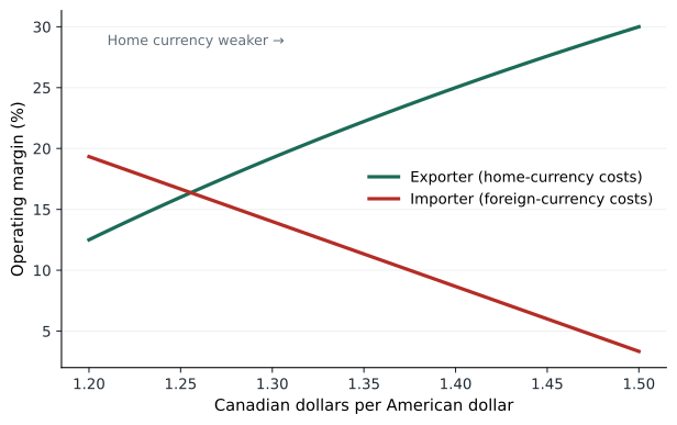
# How the exchange rate moves margins for an exporter and an importer
def exporter_margin(fx, price_usd=100.0, cost_cad=105.0):
    revenue_cad = price_usd * fx            # fx = Canadian dollars per American dollar
    return (revenue_cad - cost_cad) / revenue_cad

def importer_margin(fx, price_cad=150.0, cost_usd=80.0, other_cad=25.0):
    cost = cost_usd * fx + other_cad
    return (price_cad - cost) / price_cad

print(" CAD per USD   exporter margin   importer margin")
for fx in (1.25, 1.30, 1.35, 1.40, 1.45):
    print(f"   {fx:5.2f}        {exporter_margin(fx):7.1%}          {importer_margin(fx):7.1%}")
# Partial hedge: the importer locks in 60 % of next year's purchases at 1.35
spot = 1.45
blended = 0.6 * 1.35 + 0.4 * spot
print(f"Importer margin at spot {spot} with a 60 % hedge at 1.35: {importer_margin(blended):.1%} (unhedged {importer_margin(spot):.1%})") CAD per USD exporter margin importer margin
1.25 16.0% 16.7%
1.30 19.2% 14.0%
1.35 22.2% 11.3%
1.40 25.0% 8.7%
1.45 27.6% 6.0%
Importer margin at spot 1.45 with a 60 % hedge at 1.35: 9.2% (unhedged 6.0%)The code illustrates Grace's and Daniel's opposite exposures. Northfield sells some parts to American customers at prices in American dollars while its costs are mostly in Canadian dollars, so a weaker Canadian dollar, more Canadian dollars per American dollar, raises its margin. Fairway imports much of its produce in winter, priced in American dollars, so a weaker Canadian dollar squeezes its margin unless it raises shelf prices. Hedging with forward contracts smooths the effect for a year or so, as the last line shows, but cannot protect against a lasting change in the exchange rate; for that, firms adjust sourcing, pricing and where they produce.
Trade policy
Trade policy has become a major source of business risk. Since 2025, the United States has imposed tariffs under section 232 of its trade law on steel, aluminum, automobiles and parts, and softwood lumber, among other products, and Canada responded with retaliatory tariffs on some American goods, along with a program of tariff remission for certain inputs that Canadian manufacturers need, extended to 1 July 2027. The Canada–United States–Mexico Agreement, which kept most trade between the three countries tariff-free, came up for its joint review on 1 July 2026. The United States did not agree to extend the agreement's term, so it now moves to annual reviews while remaining in force until 2036 unless the parties decide otherwise. For managers, this means planning for a range of trade outcomes rather than a single forecast.
The economics of tariffs follow from the supply and demand tools of Lessons 2 and 5. A tariff raises the price of imports, protecting domestic producers but raising costs for buyers, including domestic manufacturers that use the imported goods as inputs. Who bears the tariff depends on elasticities: if buyers have few alternatives, they pay most of it; if foreign sellers have few other markets, they absorb part by cutting prices. For integrated supply chains like North American automotive manufacturing, in which parts cross the border several times before a vehicle is finished, tariffs compound at each crossing. Daniel's team mapped every Northfield part that crossed the border and its tariff status, then evaluated moving some machining to the plant on the other side of the border, sourcing steel domestically and sharing tariff costs with customers through surcharge clauses.
Building macro scenarios into plans
Because macroeconomic forecasts are uncertain, managers are better served by scenarios than by point forecasts. A good scenario set covers a base case and two or three plausible alternatives, such as a recession, an inflation shock or a trade disruption, each with consistent assumptions about growth, inflation, interest rates, exchange rates and the firm's specific drivers. The firm then tests its plan under each scenario and identifies early indicators, such as purchasing managers' indexes, yield curves, central bank statements and commodity prices, that signal which scenario is unfolding. Lesson 12 applies this approach to Cedarline Outdoor's capacity decision.
| Scenario | Growth | Inflation | Policy rate | Home currency | Effect on a cyclical exporter |
|---|---|---|---|---|---|
| Base case | Moderate | Near 2–3 % | Stable | Stable | Plan as budgeted |
| Energy-led inflation | Slower | Above 3 % | Rising | Mixed | Cost pressure, need surcharges |
| Recession | Negative | Falling | Cut | Weaker | Volumes down, currency cushions margin |
| Trade disruption | Slower | Higher on goods | Uncertain | Weaker | Tariff costs, supply chain changes |
Worked problem
Testing Northfield's budget against macro scenarios
Northfield's base budget assumes sales of 180 million dollars and operating profit of 14 million. Contribution margin is 30 % of sales. In a recession scenario, volume falls 15 % but a weaker Canadian dollar raises the dollar value of export sales, adding 2 % to total sales. In an inflation scenario, volume is flat but unrecovered cost increases cut the contribution margin to 27 %. What is operating profit in each scenario, assuming fixed costs are unchanged?
Show solution
- Fixed costs are 0.30 × 180 − 14 = 40 million dollars.
- Recession: sales are 180 × 0.85 × 1.02 = 156.1 million; contribution is 0.30 × 156.1 = 46.8 million; operating profit is 6.8 million.
- Inflation: contribution is 0.27 × 180 = 48.6 million; operating profit is 8.6 million.
- Both scenarios roughly halve profit, the recession through volume and the inflation shock through margin.
Answer: Operating profit falls to about 6.8 million dollars in the recession and 8.6 million in the inflation scenario. Daniel's responses differ: flexing labour and inventory for a recession, and price escalation clauses and procurement contracts for inflation.
Common mistakes
MistakeManagers should forecast the economy precisely.
InsteadThey should understand exposures and plan for scenarios, since precise forecasts are rarely reliable.
MistakeA higher nominal interest rate always means a higher real rate.
InsteadThe real rate depends on expected inflation as well.
MistakeOnly exporters and importers are exposed to exchange rates.
InsteadEconomic exposure affects any firm whose competitors, customers or suppliers are affected by currency moves.
MistakeHedging eliminates currency risk.
InsteadHedges smooth short-term effects but cannot offset a lasting change in the exchange rate.
MistakeTariffs are paid by foreign producers.
InsteadThe burden depends on elasticities; domestic buyers often bear much of it.
Summary and key terms
- GDP measures output; real GDP growth comes from labour, capital and productivity, and fluctuates in the business cycle.
- Industries differ in cyclical sensitivity; operating leverage amplifies the effect of demand swings on profit.
- Central banks target 2 % inflation and adjust policy rates to keep inflation and expectations anchored.
- Real interest rates equal nominal rates minus expected inflation; discount rates must be consistent with cash flows.
- Long-lived projects are highly sensitive to interest rates.
- Exchange rates create transaction, translation and economic exposures; hedging smooths but does not remove them.
- Trade policy and tariffs are a major source of risk; scenarios help managers plan for a range of outcomes.
- Gross domestic product
- The market value of final goods and services produced in an economy in a period.
- Output gap
- The difference between actual and potential output.
- Inflation
- A sustained rise in the general price level.
- Real interest rate
- The nominal interest rate adjusted for expected inflation.
- Policy rate
- The Bank of Canada's target for the overnight rate.
- Taylor rule
- A guide that sets the policy rate according to inflation and the output gap.
- Purchasing power parity
- The exchange rate that equalizes the cost of a basket of goods between countries.
- Economic exposure
- The effect of exchange rates on a firm's competitive position and future cash flows.
- Tariff
- A tax on imported goods.
Practice problems
Work each problem on paper first, then reveal the answer to check.
A loan carries a nominal rate of 7 % and expected inflation is 3 %. What is the approximate real rate?
Show answer
About 4 %, or exactly 1.07 / 1.03 − 1 ≈ 3.9 %.
Using the Taylor rule with a neutral real rate of 1 %, target inflation of 2 %, inflation of 4 % and an output gap of +1 %, what policy rate is suggested?
Show answer
1 + 4 + 0.5 × 2 + 0.5 × 1 = 6.5 %.
Why is Northfield's profit more cyclical than Fairway's?
Show answer
Its products can be postponed by customers and it has high operating leverage; grocery demand is stable.
Give an example of economic exposure for a firm with no foreign currency transactions.
Show answer
A domestic manufacturer competing with imports that become cheaper when the home currency strengthens.
What determines who bears the cost of a tariff?
Show answer
The elasticities of demand and supply; the less elastic side bears more.
Portfolio task: build three macro scenarios for your organization and estimate their effect on revenue, margin and cash flow.
Show answer
Answers vary.
Lesson quiz · 5 questions
Score 60% or more to complete this lesson.
Create a free account to save your progress, take quizzes and earn a certificate.