
MATH-441 · Lesson 8 of 12 · 21 min
Riemann versus Lebesgue integration
We now have two integrals on an interval. This lesson shows that the Lebesgue integral extends the Riemann integral, so that nothing learned in calculus has to be unlearned, and it answers the question that nineteenth-century analysts could not settle with Riemann's tools alone: exactly which bounded functions are Riemann integrable? Lebesgue's answer is short. A bounded function on \([a, b]\) is Riemann integrable if and only if its set of discontinuities has measure zero. We then compare improper Riemann integrals with Lebesgue integrals, look at examples that separate the two theories, and see how the fundamental theorem of calculus behaves in the new setting.
Riemann integrable implies Lebesgue integrable
Theorem 8.1. Let \(f\) be bounded and Riemann integrable on \([a, b]\). Then \(f\) is Lebesgue measurable, Lebesgue integrable, and \[\int_{[a, b]} f \, dm = \int_a^b f(x) \, dx.\]
Proof. Choose partitions \(P_1 \subseteq P_2 \subseteq \cdots\), each refining the last, with \(U(f, P_n) - L(f, P_n) \to 0\); refining keeps upper sums decreasing and lower sums increasing. For each \(P_n\) define step functions \(\ell_n\) and \(u_n\) equal on each open subinterval of \(P_n\) to the infimum and supremum of \(f\) there, and equal to \(f\) at the partition points. Then \(\ell_n \le f \le u_n\), the sequence \(\ell_n\) increases, \(u_n\) decreases, and \[\int \ell_n \, dm = L(f, P_n), \qquad \int u_n \, dm = U(f, P_n),\] since the finitely many partition points have measure zero. Let \(\ell = \lim \ell_n\) and \(u = \lim u_n\). These are measurable, \(\ell \le f \le u\), and by monotone convergence (applied to \(\ell_n - \ell_1\) and \(u_1 - u_n\), all bounded on a set of finite measure) \(\int \ell = \lim L(f, P_n)\) and \(\int u = \lim U(f, P_n)\). Both limits equal the Riemann integral, so \(\int (u - \ell) = 0\) with \(u - \ell \ge 0\), and by Corollary 6.6, \(u = \ell\) almost everywhere. Hence \(f = \ell\) a.e. Since Lebesgue measure is complete, \(f\) is measurable, and \(\int f \, dm = \int \ell \, dm = \int_a^b f\). \(\blacksquare\)
The proof used completeness of Lebesgue measure: a Riemann integrable function need not be Borel measurable. For example, the indicator of a non-Borel subset of the Cantor set is discontinuous only on the Cantor set, a null set, so by the criterion below it is Riemann integrable, with integral \(0\), but it is not Borel measurable.
Lebesgue's criterion
For \(x \in [a, b]\), define the oscillation of \(f\) at \(x\) as \[\omega_f(x) = \lim_{\delta \to 0^+} \sup\{|f(s) - f(t)| : s, t \in (x - \delta, x + \delta) \cap [a, b]\}.\] The function is continuous at \(x\) exactly when \(\omega_f(x) = 0\), so the discontinuity set is \(D = \{\omega_f > 0\} = \bigcup_k D_k\), where \(D_k = \{\omega_f \ge \frac{1}{k}\}\). Each \(D_k\) is closed: if \(\omega_f(x) < \frac{1}{k}\), there is \(\delta\) with oscillation below \(\frac{1}{k}\) on \((x - \delta, x + \delta)\), and then every point of that interval also has oscillation below \(\frac{1}{k}\).
Theorem 8.2 (Lebesgue's criterion). A bounded function \(f : [a, b] \to \mathbb{R}\) is Riemann integrable if and only if its set \(D\) of discontinuities has Lebesgue measure zero.
Proof that integrability implies \(m(D) = 0\). It suffices to show each \(m(D_k) = 0\). Given \(\varepsilon > 0\), choose a partition \(P\) with \(U(f, P) - L(f, P) < \frac{\varepsilon}{k}\). If a point of \(D_k\) lies in the open interior of a subinterval \(I_i\) of \(P\), then \(M_i - m_i \ge \frac{1}{k}\) on that subinterval. Summing over such subintervals, \(\frac{1}{k} \sum \ell(I_i) \le U(f, P) - L(f, P) < \frac{\varepsilon}{k}\), so these subintervals have total length less than \(\varepsilon\). The remaining points of \(D_k\) are partition points, finitely many. Hence \(m^*(D_k) < \varepsilon\) for every \(\varepsilon\), and \(m(D_k) = 0\).
Proof that \(m(D) = 0\) implies integrability. Let \(|f| \le M\), fix \(\varepsilon > 0\) and choose \(k\) with \(\frac{b - a}{k} < \varepsilon\). Since \(D_k\) is closed and bounded, it is compact, and since \(m(D_k) = 0\) it can be covered by finitely many open intervals \(J_1, \ldots, J_r\) of total length less than \(\varepsilon\). The set \(K = [a, b] \setminus \bigcup J_i\) is compact, and every point of \(K\) has oscillation less than \(\frac{1}{k}\), so each such point has an open neighbourhood on which \(\sup f - \inf f < \frac{1}{k}\). By compactness, finitely many of these neighbourhoods cover \(K\). Take \(P\) to be the partition formed by all endpoints of the \(J_i\) and of these neighbourhoods. Its subintervals are of two kinds: those inside some \(J_i\), with total length less than \(\varepsilon\) and \(M_i - m_i \le 2M\), and those inside a neighbourhood of a point of \(K\), with \(M_i - m_i < \frac{1}{k}\). Therefore \[U(f, P) - L(f, P) < 2M\varepsilon + \frac{1}{k}(b - a) < (2M + 1)\varepsilon.\] Since \(\varepsilon\) is arbitrary, \(f\) is Riemann integrable. \(\blacksquare\)
The criterion settles many classical questions at once. Every bounded monotone function is Riemann integrable, since its discontinuities are jumps and are countable. Every bounded function continuous except at countably many points is Riemann integrable. Products and compositions with continuous outer functions of Riemann integrable functions are Riemann integrable, because the discontinuity sets combine within a countable union of null sets. The Dirichlet function, discontinuous everywhere, is not, and neither is the indicator of a fat Cantor set, whose discontinuity set has measure \(\frac{1}{2}\).
Worked problem
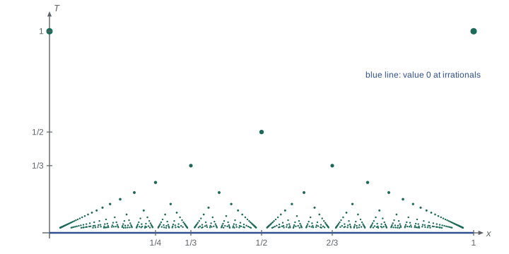
Thomae’s function
Let \(T(x) = \frac{1}{q}\) if \(x = \frac{p}{q}\) in lowest terms with \(q \ge 1\), and \(T(x) = 0\) if \(x\) is irrational, on \([0, 1]\). Find its points of continuity and decide whether it is Riemann integrable.
Show solution
- At a rational \(x = \frac{p}{q}\), \(T(x) = \frac{1}{q} > 0\), but irrationals arbitrarily close to \(x\) have \(T = 0\), so \(T\) is discontinuous at \(x\).
- At an irrational \(x\), fix \(\varepsilon > 0\). Only finitely many rationals in \([0, 1]\) have denominator \(q \le \frac{1}{\varepsilon}\), and none of them equals \(x\), so some interval around \(x\) avoids them all. On that interval \(0 \le T < \varepsilon\). So \(T\) is continuous at every irrational.
- The discontinuity set is \(\mathbb{Q} \cap [0, 1]\), which is countable, hence null. By Lebesgue’s criterion \(T\) is Riemann integrable.
- Since \(T = 0\) almost everywhere, its Lebesgue integral is \(0\), and by Theorem 8.1 so is its Riemann integral.
Answer: Thomae’s function is continuous exactly at the irrationals, Riemann integrable, and \(\int_0^1 T = 0\).
# Riemann sums for Thomae's function and for the indicator of a fat Cantor set.
from fractions import Fraction as F
from math import gcd

def thomae(x):
    """x is a Fraction (rational); irrational points give 0 and are handled separately."""
    return F(1, x.denominator)

def upper_sum_thomae(n):
    """Upper sum on the uniform partition into n pieces: sup of T on each piece over rationals."""
    total = F(0)
    for i in range(n):
        a, b = F(i, n), F(i + 1, n)
        q = 1
        while True:   # smallest denominator of a rational in [a, b]
            p_lo = -(-a.numerator * q // a.denominator)
            if F(p_lo, q) <= b:
                break
            q += 1
        total += F(1, q) * (b - a)
    return total

for n in (10, 100, 1000):
    print(f"n = {n:4d}: upper sum {float(upper_sum_thomae(n)):.5f}   lower sum 0")

# fat Cantor set S: stage-k removal of length 4^-k from each remaining interval
def fat_cantor_intervals(stages):
    ivs = [(F(0), F(1))]
    for k in range(1, stages + 1):
        new = []
        for a, b in ivs:
            mid, r = (a + b) / 2, F(1, 2 * 4 ** k)
            new += [(a, mid - r), (mid + r, b)]
        ivs = new
    return ivs

ivs = fat_cantor_intervals(12)
print("length kept after 12 stages:", float(sum(b - a for a, b in ivs)))
print("upper sum of 1_S >= m(S) = 1/2 for every partition; lower sum = 0, since S contains no interval")n = 10: upper sum 0.45667 lower sum 0 n = 100: upper sum 0.13081 lower sum 0 n = 1000: upper sum 0.03737 lower sum 0 length kept after 12 stages: 0.5001220703125 upper sum of 1_S >= m(S) = 1/2 for every partition; lower sum = 0, since S contains no interval
For the fat Cantor set \(S\), every subinterval of a partition that meets \(S\) has supremum \(1\), and these subintervals cover \(S\), so the upper sum is at least \(m(S) = \frac{1}{2}\). Every subinterval contains a removed interval, since \(S\) has empty interior, so the lower sum is \(0\). The gap never closes, in agreement with Lebesgue's criterion.
Improper integrals
The Riemann integral is defined only for bounded functions on bounded intervals; unbounded integrands and infinite intervals are handled by limits, \(\int_a^\infty f = \lim_{R \to \infty} \int_a^R f\). For nonnegative functions the two theories agree. Proposition 8.3. If \(f \ge 0\) is Riemann integrable on every \([a, R]\), then \(\int_{[a, \infty)} f \, dm = \lim_{R \to \infty} \int_a^R f\), whether the limit is finite or infinite. Proof: \(f\mathbf{1}_{[a, R]}\) increases to \(f\) as \(R \to \infty\) through the integers; apply monotone convergence and Theorem 8.1. \(\blacksquare\) The same argument handles unbounded integrands near a point, as in the example \(\int_0^1 x^{-1/2} \, dx = 2\) of lesson 6.
For functions of both signs the theories differ. If \(\int_a^\infty |f| < \infty\) as an improper integral, then \(f\) is Lebesgue integrable and the two integrals agree, by applying the proposition to \(f^+\) and \(f^-\). But a conditionally convergent improper integral, such as the Dirichlet integral \(\int_0^\infty \frac{\sin x}{x} \, dx = \frac{\pi}{2}\), has no Lebesgue counterpart, because \(\int_0^\infty \big|\frac{\sin x}{x}\big| \, dx = \infty\). One proves this by comparing with the harmonic series: on \([k\pi, (k + 1)\pi]\) the integral of \(|\sin x|\) is \(2\), and \(\frac{1}{x} \ge \frac{1}{(k+1)\pi}\) there, giving \(\int_0^{N\pi} \frac{|\sin x|}{x} \, dx \ge \frac{2}{\pi} \sum_{k=1}^{N} \frac{1}{k}\). In Lebesgue theory one writes the Dirichlet integral as \(\lim_{R \to \infty} \int_{[0, R]} \frac{\sin x}{x} \, dm\), a limit of Lebesgue integrals, much as conditionally convergent series are limits of partial sums.
What the Lebesgue integral adds
On a bounded interval, the Lebesgue integral integrates every bounded measurable function, including the Dirichlet function and the indicator of a fat Cantor set, and every measurable function with finite integral of its absolute value, bounded or not. It does not integrate conditionally convergent improper integrals, which require a limit. In return it gives the three convergence theorems, which the Riemann integral lacks, and complete function spaces, which lesson 11 builds. For computation nothing changes: whenever a function is Riemann integrable, or absolutely improperly integrable, its Lebesgue integral is computed exactly as in calculus, with antiderivatives and substitution.
A striking example of the difference comes from Vito Volterra, who in 1881 constructed a function \(V\) on \([0, 1]\) that is differentiable everywhere with a bounded derivative \(V^\prime\), but whose derivative is discontinuous on a fat Cantor set. By Lebesgue's criterion \(V^\prime\) is not Riemann integrable, so the formula \(\int_0^1 V^\prime = V(1) - V(0)\) has no meaning in Riemann's theory. In Lebesgue's theory it holds: a bounded derivative is a pointwise limit of difference quotients, hence measurable, the difference quotients are uniformly bounded by the mean value theorem, and bounded convergence gives \(\int_0^1 V^\prime \, dm = \lim_n \int_0^1 n\big(V(x + \frac{1}{n}) - V(x)\big) \, dx = V(1) - V(0)\), where \(V\) is extended to \([1, 2]\) by \(V(x) = V(1) + V^\prime(1)(x - 1)\), and the last limit holds because \(\int_0^1 n\big(V(x + \frac{1}{n}) - V(x)\big) dx = n\int_1^{1 + 1/n} V - n\int_0^{1/n} V\) and \(V\) is continuous. This was one of Lebesgue's first applications of his integral.
In the other direction, the Henstock–Kurzweil or gauge integral, developed by Jaroslav Kurzweil in 1957 and Ralph Henstock in the 1960s, modifies Riemann sums by letting the mesh vary from point to point. It integrates every derivative and every conditionally convergent improper integral, and it contains the Lebesgue integral. It has not replaced the Lebesgue integral in analysis because its integrable functions do not form a normed space with good completeness properties under the natural norm, which is precisely what the Lebesgue theory provides.
The fundamental theorem of calculus, revisited
Two versions of the fundamental theorem carry over at once. If \(f\) is continuous on \([a, b]\), then \(F(x) = \int_{[a, x]} f \, dm\) is differentiable with \(F^\prime = f\), because the integral is the Riemann integral. If \(F\) is differentiable on \([a, b]\) with \(F^\prime\) continuous, then \(\int_{[a, b]} F^\prime \, dm = F(b) - F(a)\). The general versions are more subtle. For \(f \in L^1\), the function \(F(x) = \int_a^x f\) is differentiable almost everywhere with \(F^\prime = f\) a.e.; and \(\int_a^b F^\prime = F(b) - F(a)\) holds exactly when \(F\) is absolutely continuous. The Cantor function of lesson 4 shows that differentiability almost everywhere with integrable derivative is not enough. Both theorems are discussed in the capstone.
Common mistakes
MistakeThinking every bounded function on [a, b] is Riemann integrable.
InsteadIt must be continuous except on a null set; the Dirichlet function fails.
MistakeAssuming a function continuous at no point of an interval cannot be Riemann integrable unless constant.
InsteadIntegrability needs a null discontinuity set; Thomae’s function is discontinuous on a dense set yet integrable.
MistakeTreating every convergent improper integral as a Lebesgue integral.
InsteadOnly absolutely convergent ones are; \(\int_0^\infty \frac{\sin x}{x}\) is not.
MistakeAssuming Riemann integrable functions are Borel measurable.
InsteadThey are Lebesgue measurable; an indicator of a non-Borel null set is a counterexample.
Summary and key terms
- Every Riemann integrable function on [a, b] is Lebesgue integrable with the same integral.
- Lebesgue’s criterion: a bounded function is Riemann integrable exactly when its discontinuity set has measure zero.
- Bounded monotone functions and functions with countably many discontinuities are Riemann integrable.
- Thomae’s function is continuous at irrationals, discontinuous at rationals, and integrable with integral 0.
- Nonnegative and absolutely convergent improper integrals are Lebesgue integrals; conditionally convergent ones are not.
- Lebesgue integration makes the fundamental theorem hold for every bounded derivative, including Volterra’s.
- Oscillation
- \(\omega_f(x)\), the limit of \(\sup f - \inf f\) on shrinking neighbourhoods of \(x\).
- Lebesgue’s criterion
- Riemann integrability of a bounded function is equivalent to a null set of discontinuities.
- Thomae’s function
- The function equal to 1/q at p/q in lowest terms and 0 at irrationals.
- Improper integral
- A limit of Riemann integrals over growing intervals or away from a singularity.
- Gauge integral
- The Henstock–Kurzweil integral, defined by Riemann sums with point-dependent mesh.
Practice problems
Work each problem on paper first, then reveal the answer to check.
Is \(f(x) = \sin(\frac{1}{x})\) for \(x \in (0, 1]\), \(f(0) = 0\), Riemann integrable on \([0, 1]\)?
Show answer
Yes: it is bounded and discontinuous only at 0, a null set.
Show that a bounded function with countably many discontinuities is Riemann integrable.
Show answer
Countable sets are null, so Lebesgue’s criterion applies.
Is the indicator of the middle-thirds Cantor set Riemann integrable? Find its integral.
Show answer
It is discontinuous exactly on \(C\) (points off \(C\) have neighbourhoods missing \(C\), points of \(C\) are limits of removed intervals), and \(m(C) = 0\); it is integrable with integral 0.
Evaluate \(\int_{[0, \infty)} e^{-x} \sin^2 x \, dx\) and explain why it equals the improper Riemann integral.
Show answer
The integrand is nonnegative, so Proposition 8.3 applies; using \(\sin^2 x = \frac{1 - \cos 2x}{2}\), the value is \(\frac{1}{2} - \frac{1}{2} \cdot \frac{1}{5} = \frac{2}{5}\).
Show that \(\int_1^\infty \frac{\cos x}{x^2} \, dx\) is a Lebesgue integral.
Show answer
\(\big|\frac{\cos x}{x^2}\big| \le \frac{1}{x^2}\), which has finite integral on \([1, \infty)\), so the function is Lebesgue integrable and the improper integral equals the Lebesgue one.
Lesson quiz · 5 questions
Score 60% or more to complete this lesson.
Create a free account to save your progress, take quizzes and earn a certificate.