Capstone: differentiation, Radon–Nikodym and probability

The capstone brings the course to three destinations. First, differentiation: we prove that the indefinite integral of an integrable function can be differentiated back almost everywhere, the Lebesgue differentiation theorem, and identify absolute continuity as the exact condition under which a function is the integral of its derivative. Second, the comparison of measures: the Radon–Nikodym theorem says when one measure has a density with respect to another, and the Lebesgue decomposition splits any measure into a part with a density and a singular part. Third, probability: Kolmogorov's 1933 axioms identify probability theory with measure theory on a space of total mass one, and every theorem of this course becomes a theorem about random variables. The lesson ends with a capstone project that ties the threads together.

Averages and the maximal function

For \(f \in L^1(\mathbb{R})\), let \(F(x) = \int_{-\infty}^{x} f \, dm\). If \(f\) is continuous, the fundamental theorem of calculus gives \(F^\prime = f\). For general integrable \(f\) we ask whether the averages \[A_r f(x) = \frac{1}{2r} \int_{x - r}^{x + r} f \, dm\] converge to \(f(x)\) as \(r \to 0\). Pointwise values of an element of \(L^1\) are not well defined, so the question must be almost everywhere: does \(A_r f \to f\) a.e.? The key tool is the Hardy–Littlewood maximal function \[Mf(x) = \sup_{r > 0} \frac{1}{2r} \int_{x - r}^{x + r} |f| \, dm,\] introduced by Godfrey Hardy and John Littlewood in 1930. It controls all the averages at once.

Lemma 12.1 (Vitali covering lemma, finite form). Let \(I_1, \ldots, I_n\) be bounded open intervals. There is a subcollection of pairwise disjoint intervals \(J_1, \ldots, J_k\) such that \(\bigcup_i I_i \subseteq \bigcup_j 3J_j\), where \(3J\) is the interval with the same centre and three times the length. Hence \(m\big(\bigcup I_i\big) \le 3\sum_j m(J_j)\).

Proof. Choose \(J_1\) to be a longest interval. Discard every interval that meets \(J_1\), choose \(J_2\) to be a longest remaining one, and continue until none remain. The chosen intervals are disjoint. Every discarded interval \(I\) met some chosen \(J_j\) at a step where \(J_j\) was at least as long as \(I\), so \(I \subseteq 3J_j\). \(\blacksquare\)

Theorem 12.2 (Hardy–Littlewood maximal inequality). For \(f \in L^1(\mathbb{R})\) and \(t > 0\), \[m(\{Mf > t\}) \le \frac{3}{t} \|f\|_1.\]

Proof. The set \(E_t = \{Mf > t\}\) is open, hence measurable, and by inner regularity it suffices to bound \(m(K)\) for every compact \(K \subseteq E_t\). Each \(x \in K\) is the centre of an interval \(I_x\) with \(\int_{I_x} |f| > t \, m(I_x)\). Finitely many cover \(K\); by the covering lemma, choose disjoint \(J_1, \ldots, J_k\) among them with \[m(K) \le 3\sum_j m(J_j) < \frac{3}{t}\sum_j \int_{J_j} |f| \le \frac{3}{t}\|f\|_1. \qquad \blacksquare\]

The inequality is a weak-type bound: it resembles Markov's inequality, but with \(Mf\) in place of \(|f|\), at the cost of the constant 3. It is the quantitative heart of differentiation theory, and its extensions to \(\mathbb{R}^n\) and to other families of sets are central in harmonic analysis.

The Lebesgue differentiation theorem

Theorem 12.3 (Lebesgue differentiation theorem). For \(f \in L^1(\mathbb{R})\), for almost every \(x\), \[\lim_{r \to 0} \frac{1}{2r} \int_{x - r}^{x + r} |f(y) - f(x)| \, dy = 0.\] In particular \(A_r f(x) \to f(x)\) and \(F^\prime(x) = f(x)\) for almost every \(x\).

Proof. Let \(\Omega f(x) = \limsup_{r \to 0} \frac{1}{2r}\int_{x-r}^{x+r} |f(y) - f(x)| \, dy\). We show \(m(\{\Omega f > 2t\}) = 0\) for every \(t > 0\). Fix \(\varepsilon > 0\) and, by density (Theorem 11.6), choose continuous \(g\) with compact support and \(\|f - g\|_1 < \varepsilon\). Write \(h = f - g\). Since \(g\) is continuous, \(\Omega g = 0\) everywhere, and \(\Omega f \le \Omega g + \Omega h = \Omega h \le Mh + |h|\). Hence \[\{\Omega f > 2t\} \subseteq \{Mh > t\} \cup \{|h| > t\},\] and by the maximal inequality and Markov's inequality, \(m^*(\{\Omega f > 2t\}) \le \frac{3}{t}\varepsilon + \frac{1}{t}\varepsilon\). Since \(\varepsilon\) is arbitrary, the set is null. The union over \(t = \frac{1}{n}\) is null, so \(\Omega f = 0\) a.e. Finally, \(|A_r f(x) - f(x)| \le \frac{1}{2r}\int_{x-r}^{x+r}|f - f(x)|\), and the one-sided difference quotients of \(F\) are controlled the same way. \(\blacksquare\)

Points where the conclusion holds are called Lebesgue points of \(f\). Applied to \(f = \mathbf{1}_E\) for a measurable set \(E\), the theorem gives the Lebesgue density theorem: for almost every \(x \in E\), \(\frac{m(E \cap (x - r, x + r))}{2r} \to 1\), and for almost every \(x \notin E\) the ratio tends to \(0\). A measurable set has density one at almost all of its points and density zero at almost all points outside it. There is no measurable set occupying half of every interval.

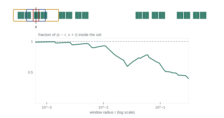
# Lebesgue density: the fraction of (x - r, x + r) covered by a fat Cantor set at a point of the set.
from fractions import Fraction as F

def fat_cantor(stages):
    ivs = [(F(0), F(1))]
    for k in range(1, stages + 1):
        new = []
        for a, b in ivs:
            mid, h = (a + b) / 2, F(1, 2 * 4 ** k)
            new += [(a, mid - h), (mid + h, b)]
        ivs = new
    return ivs

S = fat_cantor(14)
def covered(lo, hi):
    return sum(max(F(0), min(b, hi) - max(a, lo)) for a, b in S)

x = F(0)                            # 0 itself lies in every stage
for k in range(1, 9):
    r = F(1, 4 ** k)
    print(f"r = 4^-{k}: density at 0 (one-sided window) = {float(covered(x, x + r) / r):.5f}")

# a Lebesgue point test for f = 1/sqrt(|y|) at y = 0.5 (a continuity point) and at y = 0 (a singularity)
import math
def avg_dev(f, x0, r, n=20000):
    h = 2 * r / n
    return sum(abs(f(x0 - r + (i + 0.5) * h) - f(x0)) for i in range(n)) * h / (2 * r)
f = lambda y: 1 / math.sqrt(abs(y)) if y != 0 else 0.0
print("average deviation at 0.5:", [round(avg_dev(f, 0.5, 10 ** -k), 6) for k in (1, 2, 3)])
print("average deviation at 0:  ", [round(avg_dev(f, 0.0, 10 ** -k), 2) for k in (1, 2, 3)], "-> not a Lebesgue point")

r = 4^-1: density at 0 (one-sided window) = 0.61726
r = 4^-2: density at 0 (one-sided window) = 0.87701
r = 4^-3: density at 0 (one-sided window) = 0.96884
r = 4^-4: density at 0 (one-sided window) = 0.99225
r = 4^-5: density at 0 (one-sided window) = 0.99811
r = 4^-6: density at 0 (one-sided window) = 0.99957
r = 4^-7: density at 0 (one-sided window) = 0.99994
r = 4^-8: density at 0 (one-sided window) = 1.00000
average deviation at 0.5: [0.071614, 0.007072, 0.000707]
average deviation at 0:   [6.31, 19.94, 63.05] -> not a Lebesgue point

Absolute continuity and the fundamental theorem

Definition 12.4. A function \(F : [a, b] \to \mathbb{R}\) is absolutely continuous if for every \(\varepsilon > 0\) there is \(\delta > 0\) such that \(\sum_i |F(b_i) - F(a_i)| < \varepsilon\) for every finite collection of disjoint subintervals \((a_i, b_i)\) of total length less than \(\delta\).

Absolutely continuous functions are uniformly continuous (take one interval) and of bounded variation. Lipschitz functions are absolutely continuous. The Cantor function is not: the stage-\(n\) intervals have total length \((\frac{2}{3})^n\), arbitrarily small, yet the function rises by \(1\) across them. By Proposition 7.8, every indefinite integral \(F(x) = \int_a^x f\) with \(f \in L^1\) is absolutely continuous.

Theorem 12.5 (fundamental theorem of calculus for the Lebesgue integral). (a) If \(f \in L^1([a, b])\) and \(F(x) = \int_a^x f\), then \(F\) is absolutely continuous and \(F^\prime = f\) almost everywhere. (b) If \(F\) is absolutely continuous on \([a, b]\), then \(F\) is differentiable almost everywhere, \(F^\prime \in L^1\), and \(F(x) - F(a) = \int_a^x F^\prime\) for all \(x\).

Part (a) combines Proposition 7.8 with Theorem 12.3. Part (b) is deeper. Lebesgue's theorem that monotone functions are differentiable almost everywhere, together with the decomposition of a function of bounded variation as a difference of monotone functions, shows that \(F^\prime\) exists a.e. and is integrable. Then \(G = F - \int_a^x F^\prime\) is absolutely continuous with \(G^\prime = 0\) a.e., and a Vitali covering argument shows that such a function is constant. The Cantor function shows that absolute continuity cannot be weakened to continuity with derivative zero a.e. The theorem completes the story begun in lesson 8: the Lebesgue integral is exactly the right integral for recovering an absolutely continuous function from its derivative.

Absolutely continuous and singular measures

Definition 12.6. Let \(\mu, \nu\) be measures on \((X, \mathcal{A})\). Then \(\nu\) is absolutely continuous with respect to \(\mu\), written \(\nu \ll \mu\), if \(\mu(E) = 0\) implies \(\nu(E) = 0\). The measures are mutually singular, written \(\nu \perp \mu\), if there is a set \(S\) with \(\mu(S) = 0\) and \(\nu(S^c) = 0\).

If \(\nu(E) = \int_E f \, d\mu\) for some \(f \ge 0\), then \(\nu \ll \mu\), since integrals over null sets vanish. The Cantor measure \(\mu_c\) of lesson 4 is singular with respect to Lebesgue measure: it lives on the Cantor set \(C\), with \(m(C) = 0\) and \(\mu_c(C^c) = 0\). A Dirac measure \(\delta_0\) is also singular with respect to \(m\).

Theorem 12.7 (Lebesgue decomposition and Radon–Nikodym). Let \(\mu\) and \(\nu\) be σ-finite measures on \((X, \mathcal{A})\). (a) There are unique measures \(\nu_a \ll \mu\) and \(\nu_s \perp \mu\) with \(\nu = \nu_a + \nu_s\). (b) There is a measurable \(f \ge 0\), unique up to \(\mu\)-null sets, with \(\nu_a(E) = \int_E f \, d\mu\). In particular, if \(\nu \ll \mu\) then \(\nu(E) = \int_E f \, d\mu\) for all \(E\). The function \(f\) is the Radon–Nikodym derivative \(\frac{d\nu}{d\mu}\).

Proof sketch (John von Neumann's Hilbert-space argument, for finite measures). Let \(\rho = \mu + \nu\). The map \(g \mapsto \int g \, d\nu\) is a bounded linear functional on \(L^2(\rho)\), since \(\big|\int g \, d\nu\big| \le \int |g| \, d\rho \le \rho(X)^{1/2}\|g\|_{L^2(\rho)}\). By the Riesz representation theorem for Hilbert spaces, there is \(h \in L^2(\rho)\) with \(\int g \, d\nu = \int g h \, d\rho\) for all \(g\). Testing with indicators shows \(0 \le h \le 1\) \(\rho\)-a.e. Then \(\int g(1 - h) \, d\nu = \int g h \, d\mu\). Let \(S = \{h = 1\}\); taking \(g = \mathbf{1}_S\) gives \(\mu(S) = 0\), and \(\nu_s = \nu|_S\) is the singular part. On \(S^c\), take \(g = \mathbf{1}_{E \cap S^c}(1 + h + \cdots + h^n)\). Then \(\int_{E \cap S^c} (1 - h^{n+1}) \, d\nu = \int_{E \cap S^c} (h + h^2 + \cdots + h^{n+1}) \, d\mu\). As \(n \to \infty\), both integrands increase, the left one to \(1\) because \(h < 1\) on \(S^c\), so monotone convergence gives \(\nu(E \cap S^c) = \int_{E \cap S^c} \frac{h}{1 - h} \, d\mu\), and \(f = \frac{h}{1-h}\mathbf{1}_{S^c}\). The σ-finite case follows by decomposing \(X\) into pieces of finite measure. \(\blacksquare\)

Johann Radon proved the theorem for measures on \(\mathbb{R}^n\) in 1913, and Otton Nikodym extended it to abstract measure spaces in 1930; von Neumann's proof dates from 1940. The σ-finiteness of \(\mu\) is needed: counting measure \(\mu\) on \([0, 1]\) and Lebesgue measure \(m\) satisfy \(m \ll \mu\) trivially, but \(m\) has no density with respect to \(\mu\), since \(\int_{\{x\}} f \, d\mu = f(x)\) would have to equal \(m(\{x\}) = 0\) for every \(x\). On the line, combining the theorem with differentiation gives a complete picture: a finite Borel measure \(\nu\) splits as \(\nu = \nu_{ac} + \nu_{sc} + \nu_{pp}\), absolutely continuous, singular continuous (like the Cantor measure) and pure point (a sum of point masses), and the density of \(\nu_{ac}\) is the derivative of the distribution function, which exists almost everywhere.

Measure-theoretic probability

In Grundbegriffe der Wahrscheinlichkeitsrechnung (1933), Andrey Kolmogorov defined a probability space to be a measure space \((\Omega, \mathcal{F}, P)\) with \(P(\Omega) = 1\). Events are measurable sets, random variables are measurable functions, and the expectation of a random variable is its integral, \(E[X] = \int_\Omega X \, dP\). The distribution of \(X\) is the pushforward measure \(P_X(B) = P(X \in B)\) on the Borel sets, and the change-of-variables formula \(E[g(X)] = \int_{\mathbb{R}} g \, dP_X\) follows from the definition of the integral by the usual progression from indicators to simple functions to monotone limits. A random variable has a density exactly when \(P_X \ll m\), and then the density is \(\frac{dP_X}{dm}\), which is the derivative of the distribution function almost everywhere.

The dictionary between the subjects is complete. Almost everywhere is almost surely; convergence in measure is convergence in probability; Markov's inequality is the same statement; monotone and dominated convergence justify exchanging limits and expectations; Fubini's theorem gives \(E[XY] = E[X]E[Y]\) for independent integrable variables; the Borel–Cantelli lemma is the first step to the strong law of large numbers; the layer-cake formula is \(E[X] = \int_0^\infty P(X > t) \, dt\); and Hölder's inequality bounds moments. Most importantly, the Radon–Nikodym theorem defines conditional expectation: for a sub-σ-algebra \(\mathcal{G}\) and integrable \(X \ge 0\), the measure \(Q(G) = E[X\mathbf{1}_G]\) on \(\mathcal{G}\) is absolutely continuous with respect to \(P|_{\mathcal{G}}\), and its Radon–Nikodym derivative is \(E[X \mid \mathcal{G}]\), the best guess of \(X\) given the information in \(\mathcal{G}\). For \(X \in L^2\), it is the orthogonal projection of \(X\) onto the closed subspace \(L^2(\mathcal{G})\), which links the probabilistic and Hilbert-space viewpoints of lesson 11.

# Expectation as an integral: layer cake, Monte Carlo with an error estimate, and conditional expectation.
import random, math
random.seed(441)

# X exponential with rate 2: E[X] = 1/2, P(X > t) = exp(-2t)
layer = sum(math.exp(-2 * (k + 0.5) / 1000) for k in range(20000)) / 1000
print(f"layer cake: integral of P(X > t) dt = {layer:.5f}  (E[X] = 0.5)")

n = 100000
xs = [random.expovariate(2) for _ in range(n)]
mean = sum(xs) / n
sd = math.sqrt(sum((x - mean) ** 2 for x in xs) / (n - 1))
print(f"Monte Carlo mean {mean:.4f} +/- {1.96 * sd / math.sqrt(n):.4f} (95% interval)")

# strong law along one path: running means approach 1/2 almost surely
running = [sum(xs[:k]) / k for k in (10, 100, 1000, 10000, 100000)]
print("running means:", [round(r, 4) for r in running])

# conditional expectation of a die roll given low/high, as a Radon-Nikodym derivative on the atoms
die = range(1, 7)
atoms = {"low": [1, 2, 3], "high": [4, 5, 6]}
for name, A in atoms.items():
    Q, P = sum(w / 6 for w in A), len(A) / 6
    print(f"E[X | {name}] = Q(A)/P(A) = {Q / P}")

layer cake: integral of P(X > t) dt = 0.50000  (E[X] = 0.5)
Monte Carlo mean 0.4979 +/- 0.0031 (95% interval)
running means: [0.5676, 0.5105, 0.4767, 0.4957, 0.4979]
E[X | low] = Q(A)/P(A) = 2.0
E[X | high] = Q(A)/P(A) = 5.0

Capstone project

The project asks you to study one measure in depth, the distribution of a random variable built from coin tosses, using every part of the course. Let \(\varepsilon_1, \varepsilon_2, \ldots\) be independent with \(P(\varepsilon_k = 0) = P(\varepsilon_k = 2) = \frac{1}{2}\), and let \(Y = \sum_{k=1}^{\infty} \varepsilon_k 3^{-k}\).

(1) Construct the underlying probability space as a product of two-point spaces (lesson 10, with the infinite product taken on trust) and show that \(Y\) is a random variable (lesson 5). (2) Show that \(Y\) takes values in the Cantor set and that its distribution function is the Cantor function, so that \(P_Y = \mu_c\) (lesson 4). (3) Prove that \(P_Y\) has no atoms and is singular with respect to Lebesgue measure, and explain what the Lebesgue decomposition of \(P_Y\) is (this lesson). (4) Compute \(E[Y]\) and \(\operatorname{Var}(Y)\) by exchanging sum and expectation, and justify each exchange with a convergence theorem (lessons 6 and 7); the answers are \(\frac{1}{2}\) and \(\frac{1}{8}\). (5) Show that the distribution function \(c\) satisfies \(c^\prime = 0\) almost everywhere and explain why this does not contradict Theorem 12.5 (lessons 8 and 12). (6) Replace the digit choice \(\{0, 2\}\) by \(\{0, 1, 2\}\) with equal probabilities and show that the resulting distribution is Lebesgue measure on \([0, 1]\), using the π–λ uniqueness theorem (lesson 2). (7) Write a short report, in the style of a mathematical paper, with complete proofs, a figure of the distribution function, and a Python simulation estimating \(E[Y]\) and the measure of a removed interval.

The project shows how the abstract framework resolves concrete questions that the Riemann integral could not even pose. The same tools, extended to infinite-dimensional spaces, underlie stochastic processes such as Brownian motion, the ergodic theorems of dynamical systems, and the spectral theory of operators in MATH-445. Measure theory is the language in which all of modern analysis and probability is written.