
MATH-441 · Lesson 6 of 12 · 21 min
The Lebesgue integral and the monotone convergence theorem
With measurable functions and simple-function approximation in hand, we can define the Lebesgue integral. We do it in two steps. For a nonnegative simple function the integral is the obvious finite sum of values times measures. For a general nonnegative measurable function it is the supremum of the integrals of simple functions below it. The definition is short, but its consequences are deep, and the first and most important is the monotone convergence theorem, which says that integrals of increasing sequences converge to the integral of the limit with no further hypothesis. In this lesson \((X, \mathcal{A}, \mu)\) is a fixed measure space.
Integrals of simple functions
Definition 6.1. If \(\varphi = \sum_{k=1}^{n} a_k \mathbf{1}_{E_k}\) is a nonnegative simple function in canonical form, its integral is \[\int \varphi \, d\mu = \sum_{k=1}^{n} a_k \, \mu(E_k),\] with the convention \(0 \cdot \infty = 0\). For \(E \in \mathcal{A}\), \(\int_E \varphi \, d\mu = \int \varphi \mathbf{1}_E \, d\mu\).
The convention \(0 \cdot \infty = 0\) is natural: the zero function on \(\mathbb{R}\) should have integral zero, although \(m(\mathbb{R}) = \infty\). The definition uses the canonical form, but any representation gives the same answer. Lemma 6.2. If \(\varphi = \sum_{j=1}^{m} b_j \mathbf{1}_{F_j}\) with \(b_j \ge 0\) and the \(F_j\) measurable and disjoint (not necessarily the level sets), then \(\int \varphi \, d\mu = \sum_j b_j \mu(F_j)\). Proof: for each value \(a_k > 0\), a point \(x\) has \(\varphi(x) = a_k\) exactly when it lies in some \(F_j\) with \(b_j = a_k\), so \(E_k\) is the disjoint union of those \(F_j\). Additivity of \(\mu\) gives \(a_k \mu(E_k) = \sum_{j : b_j = a_k} b_j \mu(F_j)\). The sets \(F_j\) with \(b_j = 0\) contribute nothing to either side, so summing over \(k\) proves the claim. \(\blacksquare\)
Proposition 6.3. For nonnegative simple \(\varphi, \psi\) and \(c \ge 0\): (a) \(\int c\varphi = c\int\varphi\); (b) \(\int (\varphi + \psi) = \int \varphi + \int \psi\); (c) if \(\varphi \le \psi\) then \(\int \varphi \le \int \psi\); (d) \(E \mapsto \int_E \varphi \, d\mu\) is a measure on \(\mathcal{A}\).
Proof. Write \(\varphi = \sum a_j \mathbf{1}_{E_j}\) and \(\psi = \sum b_k \mathbf{1}_{F_k}\) in canonical form. The sets \(E_j \cap F_k\) are disjoint, and on each of them \(\varphi + \psi = a_j + b_k\). By Lemma 6.2, \[\int (\varphi + \psi) = \sum_{j,k} (a_j + b_k) \mu(E_j \cap F_k) = \sum_j a_j \mu(E_j) + \sum_k b_k \mu(F_k),\] using \(\sum_k \mu(E_j \cap F_k) = \mu(E_j)\). For (c), on \(E_j \cap F_k\) we have \(a_j \le b_k\) whenever the set is nonempty. Part (a) is immediate, and (d) follows from countable additivity of \(\mu\) applied to each \(E_j \cap E\). \(\blacksquare\)
Integrals of nonnegative functions
Definition 6.4. For measurable \(f : X \to [0, \infty]\), \[\int f \, d\mu = \sup\Big\{ \int \varphi \, d\mu : 0 \le \varphi \le f, \ \varphi \text{ simple} \Big\}.\] The value lies in \([0, \infty]\). For simple \(f\) it agrees with Definition 6.1 by Proposition 6.3(c). We also write \(\int f\), \(\int_X f(x) \, d\mu(x)\), and for Lebesgue measure \(\int f \, dm\) or \(\int f(x) \, dx\).
Immediate properties. If \(0 \le f \le g\) then \(\int f \le \int g\), since every simple function below \(f\) is below \(g\). If \(c \in [0, \infty)\) then \(\int cf = c \int f\). If \(E \subseteq F\) then \(\int_E f \le \int_F f\). Additivity, \(\int (f + g) = \int f + \int g\), is not obvious from the definition, because a simple function below \(f + g\) need not split as a sum of simple functions below \(f\) and \(g\). It will follow from the monotone convergence theorem.
For counting measure on \(\mathbb{N}\), every function \(f : \mathbb{N} \to [0, \infty]\) is measurable and \(\int f \, d\mu = \sum_{n=1}^{\infty} f(n)\). Indeed the simple function \(f \mathbf{1}_{\{1, \ldots, N\}}\) gives the partial sum, and any simple function below \(f\) with finite integral is supported on a finite set. So series of nonnegative terms are a special case of integrals, and theorems about integrals specialize to theorems about series. For the Dirac measure, \(\int f \, d\delta_{x_0} = f(x_0)\).
Markov's inequality and null sets
Proposition 6.5 (Markov's inequality). For measurable \(f \ge 0\) and \(t > 0\), \[\mu(\{f \ge t\}) \le \frac{1}{t} \int f \, d\mu.\] Proof: the simple function \(t \mathbf{1}_{\{f \ge t\}}\) lies below \(f\), so its integral \(t\mu(\{f \ge t\})\) is at most \(\int f\). \(\blacksquare\)
Corollary 6.6. Let \(f \ge 0\) be measurable. (a) If \(\int f < \infty\), then \(f < \infty\) almost everywhere. (b) \(\int f = 0\) if and only if \(f = 0\) almost everywhere.
Proof. (a) \(\mu(\{f = \infty\}) \le \mu(\{f \ge t\}) \le \frac{1}{t}\int f\) for every \(t\), so it is zero. (b) If \(\int f = 0\) then \(\mu(\{f \ge \frac{1}{n}\}) = 0\) for every \(n\), and \(\{f > 0\} = \bigcup_n \{f \ge \frac{1}{n}\}\) is null. Conversely, if \(f = 0\) outside a null set \(N\), every simple \(\varphi \le f\) vanishes outside \(N\), so \(\int \varphi \le (\max \varphi) \, \mu(N) = 0\). \(\blacksquare\) Part (b) is the precise sense in which the integral ignores null sets, and it is why we can identify functions equal almost everywhere.
The monotone convergence theorem
Theorem 6.7 (monotone convergence theorem). Let \(f_1, f_2, \ldots\) be measurable functions with \(0 \le f_1 \le f_2 \le \cdots\), and let \(f = \lim_n f_n\) pointwise. Then \(f\) is measurable and \[\int f \, d\mu = \lim_{n \to \infty} \int f_n \, d\mu.\]
Proof. The limit \(f = \sup_n f_n\) exists in \([0, \infty]\) and is measurable by Theorem 5.4. Monotonicity of the integral gives \(\int f_n \le \int f_{n+1} \le \int f\), so the limit \(\alpha = \lim_n \int f_n\) exists in \([0, \infty]\) and \(\alpha \le \int f\).
For the reverse inequality, fix a simple function \(\varphi\) with \(0 \le \varphi \le f\) and a number \(c \in (0, 1)\). Let \(E_n = \{x : f_n(x) \ge c\varphi(x)\}\). These sets are measurable and increase with \(n\), because the \(f_n\) increase. Their union is \(X\): if \(\varphi(x) = 0\) then \(x \in E_1\); if \(\varphi(x) > 0\) then \(c\varphi(x) < \varphi(x) \le f(x)\), so \(f_n(x) \ge c\varphi(x)\) for large \(n\). Now \[\int f_n \ge \int_{E_n} f_n \ge \int_{E_n} c\varphi = c \int_{E_n} \varphi.\] By Proposition 6.3(d), \(E \mapsto \int_E \varphi\) is a measure, so continuity from below gives \(\int_{E_n} \varphi \to \int_X \varphi\). Letting \(n \to \infty\), \(\alpha \ge c \int \varphi\). Letting \(c \to 1\), \(\alpha \ge \int \varphi\). Taking the supremum over \(\varphi\), \(\alpha \ge \int f\). \(\blacksquare\)
The factor \(c < 1\) is the clever step. Without it, the sets \(\{f_n \ge \varphi\}\) might not exhaust \(X\): at a point where \(\varphi(x) = f(x)\) and every \(f_n(x) < f(x)\), the point would never enter. Shrinking \(\varphi\) slightly guarantees that every point eventually enters.
Consequences
Corollary 6.8 (additivity). For measurable \(f, g \ge 0\), \(\int (f + g) = \int f + \int g\). Proof: take simple \(\varphi_n \uparrow f\) and \(\psi_n \uparrow g\) by Theorem 5.6. Then \(\varphi_n + \psi_n\) are simple and increase to \(f + g\), so by monotone convergence and Proposition 6.3(b), \(\int (f + g) = \lim \int (\varphi_n + \psi_n) = \lim \big(\int \varphi_n + \int \psi_n\big) = \int f + \int g\). \(\blacksquare\)
Corollary 6.9 (series of nonnegative functions). For measurable \(g_k \ge 0\), \[\int \sum_{k=1}^{\infty} g_k \, d\mu = \sum_{k=1}^{\infty} \int g_k \, d\mu.\] Proof: apply monotone convergence to the partial sums, using additivity for each finite sum. \(\blacksquare\) Term-by-term integration of nonnegative series is therefore always valid, with both sides possibly infinite. Applied to counting measure on \(\mathbb{N} \times \mathbb{N}\) organized by rows, it gives the classical theorem that a double series of nonnegative terms can be summed in either order.
Corollary 6.10. For measurable \(f \ge 0\), the function \(\nu(E) = \int_E f \, d\mu\) is a measure on \(\mathcal{A}\), and \(\int g \, d\nu = \int g f \, d\mu\) for every measurable \(g \ge 0\). Proof: for disjoint \(E_k\) with union \(E\), \(f\mathbf{1}_E = \sum_k f\mathbf{1}_{E_k}\), so Corollary 6.9 gives countable additivity. The formula for \(\int g \, d\nu\) holds for indicators by definition, for simple \(g\) by linearity, and for general \(g\) by monotone convergence. \(\blacksquare\) The function \(f\) is called the density of \(\nu\) with respect to \(\mu\), written \(d\nu = f \, d\mu\). The Radon–Nikodym theorem in lesson 12 characterizes which measures have densities.
Worked problem
An unbounded integrand
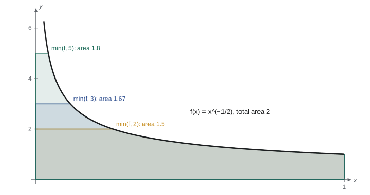
Compute \(\int_{(0, 1]} x^{-1/2} \, dx\) with respect to Lebesgue measure.
Show solution
- Let \(f_n = x^{-1/2} \mathbf{1}_{[1/n^2, 1]}\). These are nonnegative, measurable and increase pointwise to \(x^{-1/2}\) on \((0, 1]\).
- Each \(f_n\) is continuous on a closed interval, where (as lesson 8 proves) the Lebesgue and Riemann integrals agree: \(\int f_n = \int_{1/n^2}^{1} x^{-1/2} \, dx = 2 - \frac{2}{n}\).
- By monotone convergence, \(\int_{(0, 1]} x^{-1/2} \, dx = \lim_n \big(2 - \frac{2}{n}\big) = 2\).
Answer: The integral is \(2\). The improper Riemann integral is replaced by a genuine Lebesgue integral, with monotone convergence doing the work of the limit.
# Monotone convergence in action: increasing truncations of x^(-1/2) on (0, 1].
import math

def integral(g, a, b, n=200000):
    """Midpoint rule on [a, b] for a continuous integrand."""
    h = (b - a) / n
    return h * sum(g(a + (i + 0.5) * h) for i in range(n))

f = lambda x: x ** -0.5
for n in (2, 4, 16, 64, 256):
    # f_n = min(f, n) is continuous on [0, 1]; it increases to f
    fn = lambda x, n=n: min(f(x), n) if x > 0 else n
    print(f"n = {n:3d}: integral of min(f, n) = {integral(fn, 0, 1):.5f}   exact 2 - 1/n = {2 - 1 / n:.5f}")

# term-by-term integration of a nonnegative series: sum of x^k (1 - x) over k equals 1 on [0, 1)
partial = [sum(1 / ((k + 1) * (k + 2)) for k in range(N)) for N in (10, 100, 1000)]
print("sum of integrals of x^k (1 - x), partial sums:", [round(p, 4) for p in partial], "-> integral of 1 = 1")n = 2: integral of min(f, n) = 1.50000 exact 2 - 1/n = 1.50000 n = 4: integral of min(f, n) = 1.75000 exact 2 - 1/n = 1.75000 n = 16: integral of min(f, n) = 1.93750 exact 2 - 1/n = 1.93750 n = 64: integral of min(f, n) = 1.98437 exact 2 - 1/n = 1.98438 n = 256: integral of min(f, n) = 1.99609 exact 2 - 1/n = 1.99609 sum of integrals of x^k (1 - x), partial sums: [0.9091, 0.9901, 0.999] -> integral of 1 = 1
In the code, the truncations \(\min(f, n)\) are bounded and continuous, so a Riemann sum computes their integrals reliably; the exact value is \(\int_0^{1/n^2} n \, dx + \int_{1/n^2}^1 x^{-1/2} \, dx = \frac{1}{n} + 2 - \frac{2}{n} = 2 - \frac{1}{n}\). For the series, \(\int_0^1 x^k (1 - x) \, dx = \frac{1}{(k + 1)(k + 2)}\), and the sum telescopes to \(1\), which is the integral of \(\sum_k x^k(1 - x) = 1\) on \([0, 1)\).
Monotone convergence for decreasing sequences
The theorem has no direct analogue for decreasing sequences. With Lebesgue measure on \(\mathbb{R}\), \(f_n = \mathbf{1}_{[n, \infty)}\) decreases to \(0\), but every \(\int f_n = \infty\). The statement is true if \(\int f_1 < \infty\): apply monotone convergence to the increasing sequence \(f_1 - f_n\) and subtract, which requires the finiteness. This is the integral version of continuity from above, and the counterexample is the same as in lesson 2. The general tool for sequences that are not monotone is Fatou's lemma, the subject of lesson 7.
A further subtlety concerns almost everywhere hypotheses. If \(0 \le f_n \le f_{n+1}\) holds only almost everywhere and \(f_n \to f\) almost everywhere, the conclusion still holds: modify all functions to be zero on the null set where something fails, which changes no integral by Corollary 6.6. Most convergence theorems are stated with almost everywhere hypotheses for this reason, and we will do so from now on without further comment.
Common mistakes
MistakeUsing \(0 \cdot \infty = \infty\) when integrating simple functions.
InsteadThe convention is \(0 \cdot \infty = 0\), so the zero function on \(\mathbb{R}\) has integral zero.
MistakeApplying monotone convergence to a decreasing sequence without checking finiteness.
Instead\(\mathbf{1}_{[n, \infty)}\) decreases to 0 while every integral is infinite.
MistakeAssuming additivity of the integral follows directly from the definition.
InsteadIt is proved through simple-function approximation and monotone convergence.
MistakeThinking an infinite integral means the function is infinite somewhere.
InsteadThe constant 1 on \(\mathbb{R}\) is finite everywhere and has infinite integral; only finite integral forces finiteness a.e.
Summary and key terms
- For simple \(\varphi = \sum a_k \mathbf{1}_{E_k} \ge 0\), \(\int \varphi = \sum a_k \mu(E_k)\), independent of the representation.
- For measurable \(f \ge 0\), \(\int f\) is the supremum of the integrals of simple functions below \(f\).
- Markov: \(\mu(f \ge t) \le \frac{1}{t}\int f\); hence \(\int f = 0\) exactly when \(f = 0\) a.e.
- Monotone convergence: if \(0 \le f_n \uparrow f\), then \(\int f_n \to \int f\), with no other hypothesis.
- Consequences: additivity, term-by-term integration of nonnegative series, and measures defined by densities.
- Integrals with respect to counting measure are sums of series; with respect to a Dirac measure, point evaluations.
- Lebesgue integral
- For a nonnegative measurable function, the supremum of integrals of simple functions below it.
- Markov inequality
- \(\mu(\{f \ge t\}) \le \frac{1}{t}\int f \, d\mu\) for \(f \ge 0\).
- Monotone convergence theorem
- For an increasing sequence of nonnegative measurable functions, the integral of the limit is the limit of the integrals.
- Density
- A function \(f \ge 0\) with \(\nu(E) = \int_E f \, d\mu\) for all measurable \(E\).
- Almost everywhere equality
- Agreement outside a null set; it leaves integrals unchanged.
Practice problems
Work each problem on paper first, then reveal the answer to check.
Compute \(\int \varphi \, dm\) for \(\varphi = 3\mathbf{1}_{[0, 2]} + 2\mathbf{1}_{[1, 4]}\).
Show answer
Canonical form: \(3\) on \([0,1)\), \(5\) on \([1, 2]\), \(2\) on \((2, 4]\); the integral is \(3 + 5 + 4 = 12\), equal to \(3 \cdot 2 + 2 \cdot 3\).
Show that \(\int_{[1, \infty)} x^{-2} \, dx = 1\) using monotone convergence.
Show answer
\(f_n = x^{-2}\mathbf{1}_{[1, n]}\) increase to \(x^{-2}\) with integrals \(1 - \frac{1}{n} \to 1\).
Use Corollary 6.9 to show \(\int_0^1 \frac{-\ln(1 - x)}{x} \, dx = \frac{\pi^2}{6}\).
Show answer
\(\frac{-\ln(1-x)}{x} = \sum_{k \ge 1} \frac{x^{k-1}}{k}\), all terms nonnegative; integrating term by term gives \(\sum \frac{1}{k^2}\).
If \(f \ge 0\) and \(\int f = 5\), give an upper bound for \(\mu(\{f \ge 10\})\).
Show answer
Markov gives \(\mu(\{f \ge 10\}) \le \frac{5}{10} = \frac{1}{2}\).
Let \(f_n = \frac{1}{n}\mathbf{1}_{[0, n]}\). Do the integrals converge to the integral of the limit?
Show answer
\(f_n \to 0\) uniformly but \(\int f_n = 1\). The sequence is not increasing, so monotone convergence does not apply, and the conclusion fails.
Lesson quiz · 5 questions
Score 60% or more to complete this lesson.
Create a free account to save your progress, take quizzes and earn a certificate.