Measurable functions and simple-function approximation

To integrate a function in the Lebesgue manner we must be able to measure the sets \(\{x : a \le f(x) < b\}\) on which its values lie in a band. Functions for which these sets are always measurable are called measurable functions, and they are the objects of integration theory. This lesson defines them, shows that the class is closed under every operation analysis needs, including pointwise limits, and proves the key approximation theorem: every nonnegative measurable function is the increasing limit of simple functions, which take finitely many values. That theorem is the bridge to the integral in lesson 6.

Definition

Throughout, \((X, \mathcal{A})\) is a measurable space. It is convenient to allow the values \(\pm\infty\), so we work with the extended real line \(\overline{\mathbb{R}} = [-\infty, \infty]\), whose Borel sets are those generated by the intervals \((a, \infty]\).

Definition 5.1. A function \(f : X \to \overline{\mathbb{R}}\) is measurable (with respect to \(\mathcal{A}\)) if \(\{x : f(x) > a\} \in \mathcal{A}\) for every \(a \in \mathbb{R}\). When \(X = \mathbb{R}\) and \(\mathcal{A}\) is the Lebesgue σ-algebra, we say Lebesgue measurable; when \(\mathcal{A}\) is the Borel σ-algebra, Borel measurable.

Proposition 5.2. The following are equivalent for \(f : X \to \overline{\mathbb{R}}\): (a) \(\{f > a\} \in \mathcal{A}\) for all \(a\); (b) \(\{f \ge a\} \in \mathcal{A}\) for all \(a\); (c) \(\{f < a\} \in \mathcal{A}\) for all \(a\); (d) \(\{f \le a\} \in \mathcal{A}\) for all \(a\); (e) \(f^{-1}(B) \in \mathcal{A}\) for every Borel set \(B \subseteq \overline{\mathbb{R}}\).

Proof. (a) implies (b) because \(\{f \ge a\} = \bigcap_n \{f > a - \frac{1}{n}\}\). (b) implies (c) by complements, (c) implies (d) because \(\{f \le a\} = \bigcap_n \{f < a + \frac{1}{n}\}\), and (d) implies (a) by complements. For (e), the collection of sets \(B\) with \(f^{-1}(B) \in \mathcal{A}\) is a σ-algebra, because preimages commute with complements and countable unions. By (a) it contains the generators \((a, \infty]\), so it contains every Borel set. Conversely (e) implies (a) trivially. \(\blacksquare\)

This proof uses the generating-family principle from lesson 2, and condition (e) is the definition used in probability: a random variable is a measurable function on a probability space, and \(P(f \in B)\) makes sense for every Borel set \(B\). The function \(B \mapsto \mu(f^{-1}(B))\) is a measure on the Borel sets, the distribution or pushforward of \(\mu\) under \(f\).

Examples. Every continuous function \(f : \mathbb{R} \to \mathbb{R}\) is Borel measurable, since \(\{f > a\}\) is open. Every monotone function is Borel measurable, since \(\{f > a\}\) is an interval. The indicator function \(\mathbf{1}_E\) is measurable exactly when \(E\) is measurable, because \(\{\mathbf{1}_E > a\}\) is \(X\), \(E\) or \(\varnothing\). In particular, the indicator of a Vitali set is a function that is not Lebesgue measurable, and it is the kind of function that Lebesgue integration must exclude.

Operations preserve measurability

Theorem 5.3. Let \(f, g\) be measurable real-valued functions and \(c \in \mathbb{R}\). Then \(f + g\), \(cf\), \(fg\), \(\max(f, g)\), \(\min(f, g)\) and \(|f|\) are measurable. If \(\varphi : \mathbb{R} \to \mathbb{R}\) is Borel measurable, in particular continuous, then \(\varphi \circ f\) is measurable.

Proof. For sums, \(f(x) + g(x) > a\) if and only if there is a rational \(q\) with \(f(x) > q\) and \(g(x) > a - q\). Hence \[\{f + g > a\} = \bigcup_{q \in \mathbb{Q}} \big(\{f > q\} \cap \{g > a - q\}\big),\] a countable union of measurable sets. The density of the rationals is what turns an uncountable condition into a countable one. For compositions, \((\varphi \circ f)^{-1}(B) = f^{-1}(\varphi^{-1}(B))\), and \(\varphi^{-1}(B)\) is Borel when \(B\) is. Taking \(\varphi(t) = t^2\) shows \(f^2\) is measurable, and then \(fg = \frac{1}{4}\big((f + g)^2 - (f - g)^2\big)\). For maxima, \(\{\max(f, g) > a\} = \{f > a\} \cup \{g > a\}\), and \(|f| = \max(f, -f)\). \(\blacksquare\)

A warning about compositions: if \(\varphi\) is only Lebesgue measurable, \(\varphi \circ f\) need not be Lebesgue measurable, even for continuous \(f\). The function \(h^{-1}\) built from the Cantor function in lesson 4 is continuous, and the indicator of the non-Borel null set \(A\) composed with \(h^{-1}\) is the indicator of \(h(A) = V\), which is not measurable. This is one reason Borel measurability is the natural requirement for the outer function.

Theorem 5.4. If \(f_1, f_2, \ldots\) are measurable functions into \(\overline{\mathbb{R}}\), then \(\sup_n f_n\), \(\inf_n f_n\), \(\limsup_n f_n\) and \(\liminf_n f_n\) are measurable. In particular, a pointwise limit of measurable functions, where it exists, is measurable.

Proof. \(\{\sup_n f_n > a\} = \bigcup_n \{f_n > a\}\), and \(\inf_n f_n = -\sup_n(-f_n)\). Then \(\limsup_n f_n = \inf_k \sup_{n \ge k} f_n\) and \(\liminf_n f_n = \sup_k \inf_{n \ge k} f_n\). If \(f_n \to f\) pointwise then \(f = \limsup f_n\). \(\blacksquare\)

This is the property that the Riemann integrable functions lacked in lesson 1. The Dirichlet function is the pointwise limit of indicators of finite sets, each measurable, so it is measurable. In fact the class of Borel measurable functions is the smallest class containing the continuous functions and closed under pointwise limits of sequences, a characterization due to René Baire and Lebesgue.

Almost everywhere

When \(\mu\) is a measure on \(\mathcal{A}\), we usually identify functions that agree almost everywhere, since they will have the same integral. If \(\mu\) is complete, as Lebesgue measure is, then a function equal a.e. to a measurable function is itself measurable: if \(g = f\) outside a null set \(N\), then \(\{g > a\}\) differs from \(\{f > a\}\) by a subset of \(N\). Similarly, if \(f_n \to f\) almost everywhere and each \(f_n\) is measurable, \(f\) is measurable. Without completeness these statements need small modifications, which is one reason Lebesgue measure is usually preferred to Borel measure in analysis.

Simple functions

Definition 5.5. A simple function is a measurable function \(\varphi : X \to \mathbb{R}\) taking only finitely many values. If its distinct values are \(a_1, \ldots, a_n\) and \(E_k = \varphi^{-1}(a_k)\), then the sets \(E_k\) are measurable and disjoint with union \(X\), and \[\varphi = \sum_{k=1}^{n} a_k \mathbf{1}_{E_k}.\] This is the canonical form of \(\varphi\).

Step functions, which are constant on finitely many intervals, are simple functions, but simple functions are far more general: \(\mathbf{1}_{\mathbb{Q}}\) and the indicator of a fat Cantor set are simple. Sums, products, maxima and minima of simple functions are simple, since they take finitely many values on the common refinement of the partitions.

The approximation theorem

Theorem 5.6. Let \(f : X \to [0, \infty]\) be measurable. There are simple functions \(0 \le \varphi_1 \le \varphi_2 \le \cdots \le f\) with \(\varphi_n(x) \to f(x)\) for every \(x\). The convergence is uniform on every set where \(f\) is bounded.

Proof. For \(n \ge 1\) and \(k = 1, \ldots, n2^n\), let \[E_{n,k} = \Big\{ \frac{k - 1}{2^n} \le f < \frac{k}{2^n} \Big\}, \qquad F_n = \{f \ge n\},\] and define \[\varphi_n = \sum_{k=1}^{n 2^n} \frac{k - 1}{2^n} \mathbf{1}_{E_{n,k}} + n \mathbf{1}_{F_n}.\] These sets are measurable, so \(\varphi_n\) is simple, and \(0 \le \varphi_n \le f\) by construction. Each step from \(n\) to \(n + 1\) halves the band width, splitting each band \(E_{n,k}\) into two bands of \(\varphi_{n+1}\) whose values are at least \(\frac{k-1}{2^n}\), and replaces the value \(n\) on \(F_n\) by values at least \(n\); hence \(\varphi_n \le \varphi_{n+1}\). If \(f(x) < \infty\), then once \(n > f(x)\) we have \(0 \le f(x) - \varphi_n(x) < 2^{-n}\). If \(f(x) = \infty\), then \(\varphi_n(x) = n \to \infty\). On a set where \(f \le M\), the error is less than \(2^{-n}\) for all \(n > M\), uniformly. \(\blacksquare\)

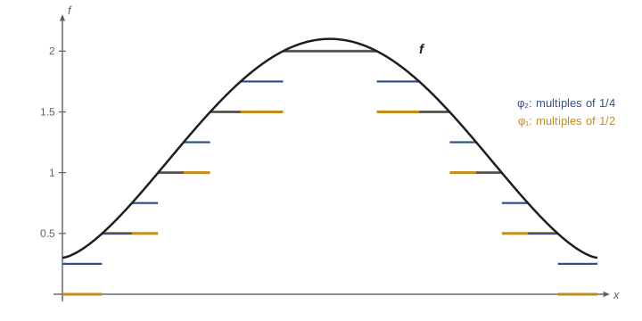
The construction rounds \(f\) down to a dyadic grid in its range, just as the Lebesgue sum of lesson 1 did. For a function of either sign, apply the theorem to the positive and negative parts \(f^+ = \max(f, 0)\) and \(f^- = \max(-f, 0)\), which are measurable and satisfy \(f = f^+ - f^-\) and \(|f| = f^+ + f^-\). Then \(\varphi_n^+ - \varphi_n^-\) is a sequence of simple functions converging to \(f\) with \(|\varphi_n^+ - \varphi_n^-| \le |f|\).

# Dyadic simple-function approximation: phi_n rounds f down to a multiple of 2^-n, capped at n.
import math

def phi(n, y):
    if y >= n:
        return float(n)
    return math.floor(y * 2 ** n) / 2 ** n

f = lambda x: 1 / math.sqrt(x) if x > 0 else math.inf     # unbounded near 0
grid = [i / 10000 for i in range(1, 10001)]

for n in (1, 2, 4, 8, 12):
    err_bounded = max(f(x) - phi(n, f(x)) for x in grid if f(x) <= 3)
    values = sorted({phi(n, f(x)) for x in grid})
    print(f"n = {n:2d}: {len(values):5d} distinct values, max error where f <= 3: {err_bounded:.5f}  (bound 2^-n = {2 ** -n:.5f})")

# monotonicity check at a few points
for x in (0.001, 0.2, 0.9):
    print(x, [round(phi(n, f(x)), 4) for n in range(1, 7)])

n =  1:     1 distinct values, max error where f <= 3: 1.99880  (bound 2^-n = 0.50000)
n =  2:     5 distinct values, max error where f <= 3: 0.99880  (bound 2^-n = 0.25000)
n =  4:    49 distinct values, max error where f <= 3: 0.06250  (bound 2^-n = 0.06250)
n =  8:  1230 distinct values, max error where f <= 3: 0.00391  (bound 2^-n = 0.00391)
n = 12:  6259 distinct values, max error where f <= 3: 0.00024  (bound 2^-n = 0.00024)
0.001 [1.0, 2.0, 3.0, 4.0, 5.0, 6.0]
0.2 [1.0, 2.0, 2.125, 2.1875, 2.2188, 2.2344]
0.9 [1.0, 1.0, 1.0, 1.0, 1.0312, 1.0469]

Littlewood's second principle: Lusin's theorem

Measurable functions can be wildly discontinuous, like the Dirichlet function, but they are nearly continuous in a measure-theoretic sense. Theorem 5.7 (Lusin, 1912). Let \(f : [a, b] \to \mathbb{R}\) be Lebesgue measurable and \(\varepsilon > 0\). There is a closed set \(F \subseteq [a, b]\) with \(m([a, b] \setminus F) < \varepsilon\) such that the restriction \(f|_F\) is continuous.

Proof sketch. First suppose \(f\) is simple, \(f = \sum a_k \mathbf{1}_{E_k}\) in canonical form. By regularity (lesson 3), choose closed sets \(F_k \subseteq E_k\) with \(m(E_k \setminus F_k) < \frac{\varepsilon}{n}\). On \(F = \bigcup F_k\), a finite union of disjoint closed sets, \(f\) is constant on each piece, and the pieces are at positive distance from each other, so \(f|_F\) is continuous. For general \(f\), first reduce to bounded \(f\) by discarding the set \(\{|f| > M\}\) of small measure. Then take simple \(\varphi_n\) converging uniformly to \(f\), find closed sets \(F_n\) with \(m([a, b] \setminus F_n) < \varepsilon 2^{-n}\) on which \(\varphi_n\) is continuous, and let \(F = \bigcap F_n\). On \(F\), \(f\) is a uniform limit of continuous functions, hence continuous, and \(m([a, b] \setminus F) < \varepsilon\). \(\blacksquare\)

The theorem says the restriction of \(f\) to \(F\) is continuous, not that \(f\) is continuous at points of \(F\). For the Dirichlet function, \(F\) can be taken to be a closed set of irrationals of measure close to \(b - a\), on which the function is identically zero; yet the function is discontinuous at every point. By the Tietze extension theorem the restriction can be extended to a continuous function \(g\) on \([a, b]\) with \(f = g\) outside a set of measure less than \(\varepsilon\), and with \(\sup |g| \le \sup |f|\).

The translation of quantifiers into set operations in this example is a skill worth practising. As long as all quantifiers range over countable sets, the result is measurable. Quantifiers over uncountable sets, such as all real \(\varepsilon > 0\), can usually be replaced by countable ones, such as \(\varepsilon = \frac{1}{j}\), using monotonicity in the parameter.